Process Concept
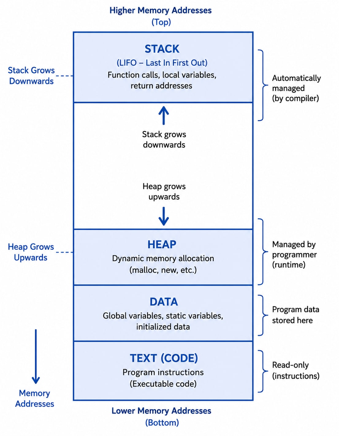
A process is a program that is currently being executed. When a program starts running, it becomes a process. It performs the tasks written in the program one after another. In simple words, we write a program in a programming language and save it as a file. When the operating system loads that program into memory and starts executing it, the program becomes a process. A process is stored in memory in different sections, each having a specific purpose.
-
Stack - The Stack stores temporary data required while the program is running, such as function parameters, local variables, and return addresses.
-
Heap - The Heap is used for memory that is allocated dynamically during the execution of a program. The programmer can request and release this memory whenever needed.
-
Data Section - The Data section stores all the global and static variables used by the program.
-
Text (Code) Section - The Text section contains the executable instructions of the program. It also includes information required by the CPU, such as the Program Counter, which keeps track of the next instruction to execute.
Program
A program is a collection of instructions written in a programming language to perform a specific task. It can be as small as a few lines of code or as large as millions of lines.
For example, the following C program prints "Hello, World!" on the screen.
#include <stdio.h>

int main() {
    printf("Hello, World!\n");
    return 0;
}
A program is stored on a storage device such as a hard disk or SSD and does nothing until it is executed.When a program starts running, it becomes a process. Therefore, a process is simply a running instance of a program.An algorithm is a step-by-step procedure used to solve a problem or perform a specific task.A collection of programs, libraries, and related files is called software.
Process Life Cycle
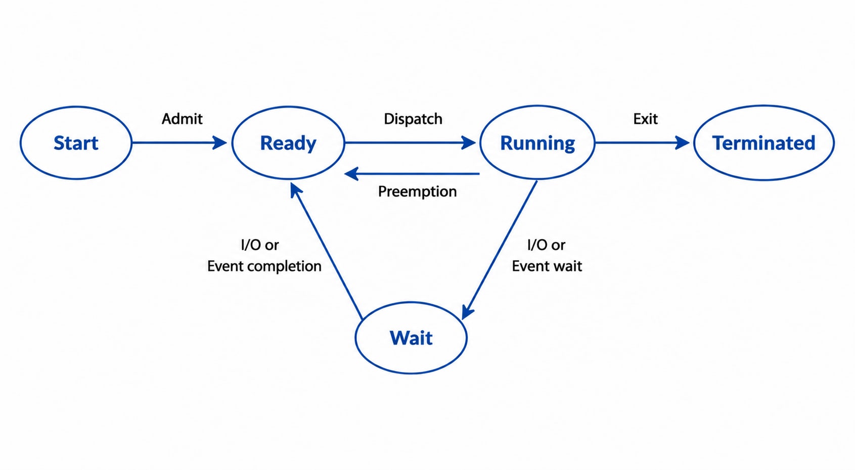
A process goes through different stages from the time it starts until it finishes. These stages are called process states. Although different operating systems may use slightly different names, the basic states are almost the same.
-
New (Start) - This is the first state of a process. The operating system creates the process and prepares it for execution.
-
Ready - In this state, the process is ready to run but is waiting for the CPU. The operating system scheduler decides when the CPU will be assigned to it.A process may enter the Ready state after being created or after being interrupted while running.
-
Running - Once the CPU is assigned to the process, it enters the Running state. The CPU executes the instructions of the process in this state.
-
Waiting (Blocked) - A process enters the Waiting state when it cannot continue until a particular event occurs, such as receiving user input or completing an I/O operation.
-
Terminated (Exit) - When the process completes its execution or is stopped by the operating system, it enters the Terminated state. After that, its resources are released from memory.
Process Control Block (PCB)
A Process Control Block (PCB) is a data structure maintained by the operating system for every process. It stores all the information needed to manage and control a process. Each process has its own unique Process ID (PID), which helps the operating system identify it.
The PCB contains the following information:
-
Process State - Stores the current state of the process, such as Ready, Running, Waiting, or Terminated.
-
Process Privileges - Stores the permissions that determine which system resources the process can access.
-
Process ID (PID) - A unique number assigned to every process.
-
Parent Process Pointer - Stores a reference to the parent process that created the current process.
-
Program Counter (PC) - Stores the address of the next instruction that the CPU will execute.
-
CPU Registers - Stores the values of CPU registers so the process can continue execution correctly after a context switch.
-
CPU Scheduling Information - Stores scheduling details such as process priority and other information used by the CPU scheduler.
-
Memory Management Information - Stores details about the memory assigned to the process, including page tables, segment tables, and memory limits.
-
Accounting Information - Stores information such as CPU usage, execution time, process owner, and other statistics.
-
I/O Status Information - Stores information about the input/output devices and files being used by the process.
Process Scheduling
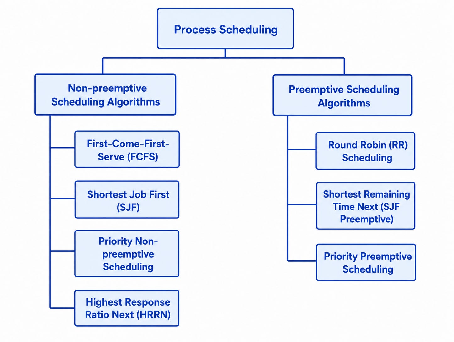
Process scheduling is the process used by the operating system to decide which process should use the CPU next. When one process finishes using the CPU or is interrupted, the process scheduler removes it from the CPU and selects another process based on a scheduling algorithm or strategy.
Process scheduling is an important feature of multiprogramming operating systems. In a multiprogramming system, more than one process can be loaded into memory at the same time. Since only one process can use the CPU at a time (for a single CPU core), the operating system shares the CPU among different processes using time multiplexing (time sharing). This helps improve CPU utilization and allows multiple programs to run efficiently.
Categories of Scheduling
There are two main types of process scheduling.
Non-Preemptive Scheduling
In Non-Preemptive Scheduling, once a process gets the CPU, it continues running until it completes its execution or enters the waiting state (for example, while waiting for an I/O operation). The operating system cannot take the CPU away from the process before it finishes or blocks itself. This means the running process keeps using the CPU without interruption. Only after the process completes or moves to the waiting state does the operating system assign the CPU to another process.
Advantages
- Easy to implement.
- Fewer context switches, so there is less overhead.
- Suitable for simple operating systems.
Disadvantages
- A long process can keep the CPU for a long time.
- Short processes may have to wait for a long time.
- Response time is slower.
Non-preemptive scheduling Algorithims
FCFS Scheduling
FCFS (First Come, First Served) is the simplest CPU scheduling algorithm. In this algorithm, the process that requests the CPU first is executed first. It follows the FIFO (First In, First Out) principle, where processes are handled in the order they arrive. FCFS is a non-preemptive scheduling algorithm. This means that once a process gets the CPU, it continues executing until it finishes or requests an I/O operation. The CPU is not taken away from the running process until it voluntarily releases it.
Features of FCFS Scheduling
- FCFS is a non-preemptive scheduling algorithm.
- The process that arrives first in the ready queue gets the CPU first.
- It is simple to understand and easy to implement.
- No information about process priority or execution time is required.
- Changes in a process's execution time do not affect the scheduling order.
- Every process gets a fair chance because execution follows the order of arrival.
- However, it may cause long waiting times for processes that arrive after a long-running process.
Real-Life Example of FCFS Scheduling
A shopping mall billing counter is a good example of FCFS scheduling. Customers are served in the same order in which they join the queue. The customer who arrives first gets billed first, followed by the next customer, and so on.
If there is no special priority for VIP customers, everyone waits for their turn. Similarly, in FCFS scheduling, the CPU executes the first process in the ready queue completely before moving to the next one. Since FCFS is non-preemptive, no newly arriving or more important process can interrupt the currently running process.
Important Terms Used in FCFS Scheduling
The following terms are commonly used while solving CPU scheduling problems.
-
Arrival Time () - Arrival Time is the time at which a process enters the ready queue.
-
Burst Time () - Burst Time, also called CPU Time, is the amount of CPU time required by a process to complete its execution.
-
Completion Time () - Completion Time is the time at which a process finishes its execution.
-
Turnaround Time () - Turnaround Time is the total time taken by a process from its arrival until completion.
Formula: or
-
Waiting Time () - Waiting Time is the total time a process spends waiting in the ready queue before getting the CPU.
Formula:
-
Response Time () - Response Time is the time from a process's arrival until it gets the CPU for the first time. In non-preemptive scheduling algorithms like FCFS, Response Time is generally equal to Waiting Time.
-
Gantt Chart - A Gantt Chart is a graphical representation of process execution. It shows the order in which processes are executed by the CPU and helps calculate scheduling parameters such as Completion Time, Turnaround Time, and Waiting Time.
Problem 1
Consider the following processes and calculate Completion Time (), Turnaround Time (), Waiting Time (), Response Time (), Average Turnaround Time, and Average Waiting Time.
Solution:
GANTT CHART:
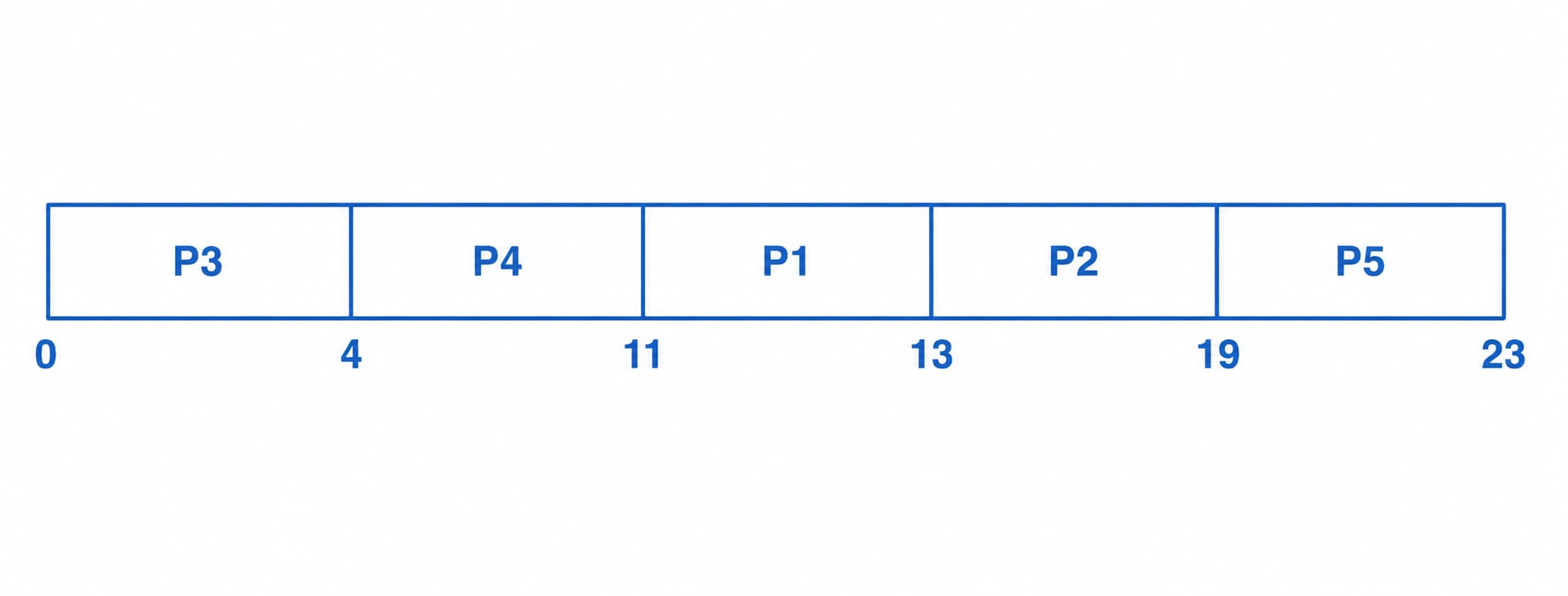
Process P1 2 2 13 11 9 9 P2 5 6 19 14 8 8 P3 0 4 4 4 0 0 P4 0 7 11 11 4 4 P5 7 4 23 16 12 12 Average Waiting Time
= (9 + 8 + 0 + 4 + 12) / 5
= 33 / 5
= 6.6 time units (for example, milliseconds)
Average Turnaround Time
= (11 + 14 + 4 + 11 + 16) / 5
= 56 / 5
= 11.2 time units (for example, milliseconds)
Problem 2
Consider the following processes and calculate Completion Time (), Turnaround Time (), Waiting Time (), Response Time (), Average Turnaround Time, and Average Waiting Time.
Solution:
GANTT CHART:
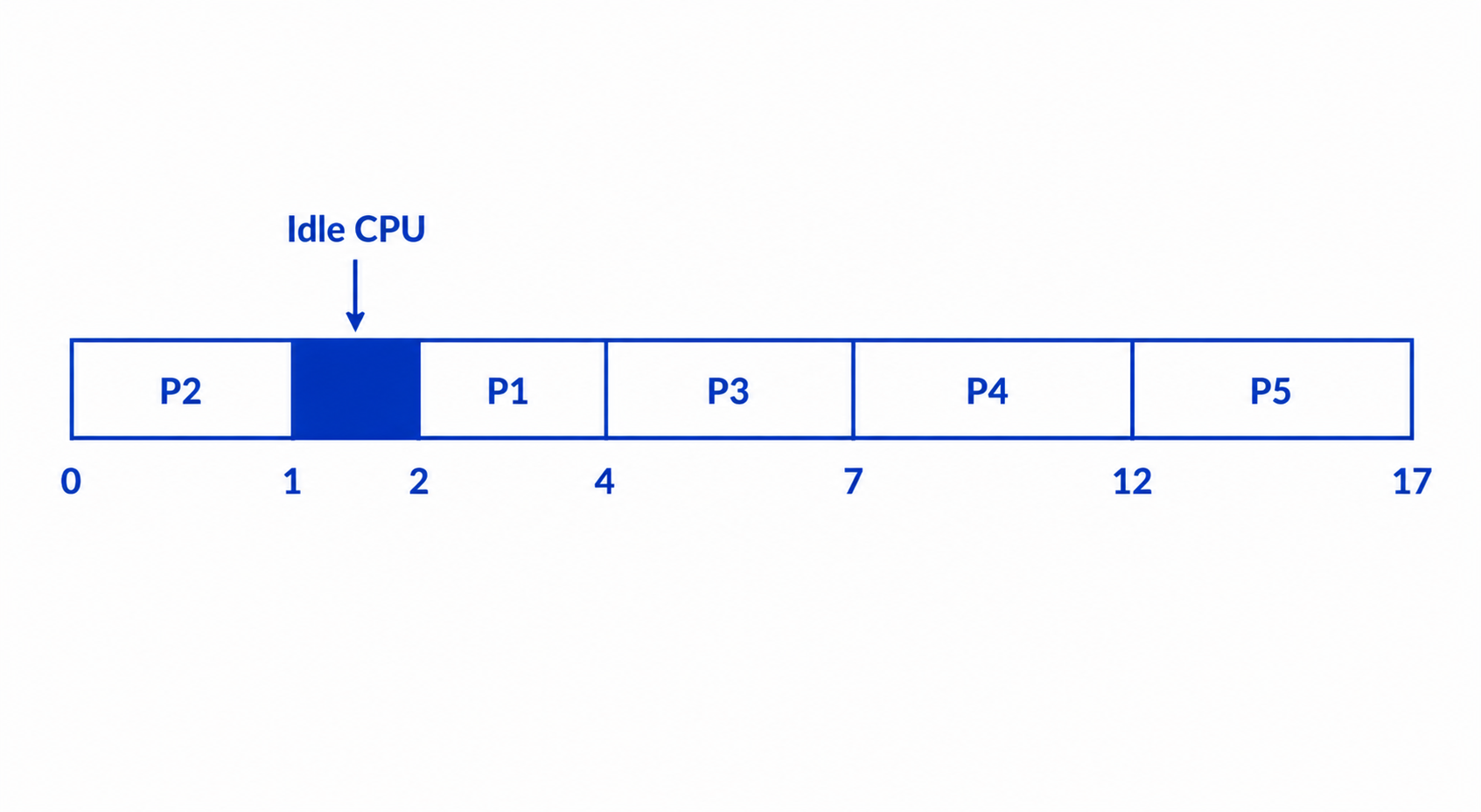
Process P1 2 2 4 2 0 0 P2 0 1 1 1 0 0 P3 2 3 7 5 2 2 P4 3 5 12 9 4 4 P5 4 5 17 13 8 8 Average Waiting Time
= (0 + 0 + 2 + 4 + 8) / 5
= 14 / 5
= 2.8 time units (for example, milliseconds)
Average Turnaround Time
= (2 + 1 + 5 + 9 + 13) / 5
= 30 / 5
= 6 time units (for example, milliseconds)
Note: During an idle CPU period, no process is available in the ready queue for execution. Therefore, the CPU remains idle until a new process arrives.
Advantages of FCFS Scheduling
- It is simple and easy to implement.
- Processes are executed in the order they arrive, following the FIFO principle.
- Every process gets a fair chance because no priority is given to any process.
- It has very low scheduling overhead.
Disadvantages of FCFS Scheduling
- FCFS may suffer from the convoy effect. If a process with a long burst time arrives first, all shorter processes have to wait until it finishes.
- Short processes may experience long waiting times because they cannot bypass longer processes.
- It is not suitable for time-sharing or interactive systems where quick response is required.
- Since it is non-preemptive, the CPU cannot interrupt a running process, even if a higher-priority process arrives.
SJF Scheduling
Shortest Job First (SJF) is a CPU scheduling algorithm in which the process with the shortest CPU burst time is selected for execution first. The scheduler always chooses the process that requires the least execution time, which helps reduce the average waiting time.
Types of SJF Scheduling
There are two types of SJF scheduling:
-
Non-Preemptive SJF - In the non-preemptive version, once a process is assigned to the CPU, it continues executing until it finishes. The CPU cannot be taken away from the running process, even if another process with a shorter burst time arrives.
The scheduler selects a new process only when:
- The currently running process completes its execution.
- The ready queue is empty and a new process arrives.
-
Preemptive SJF (Shortest Remaining Time First - SRTF) - The preemptive version of SJF is called Shortest Remaining Time First (SRTF). In SRTF, if a new process arrives with a shorter remaining execution time than the currently running process, the CPU is immediately assigned to the new process. The interrupted process is moved back to the ready queue and resumes execution later.
The scheduler is invoked whenever:
- A new process arrives.
- The currently running process completes its execution.
Features of SJF Scheduling
- The CPU is allocated to the process with the shortest burst time.
- If two or more processes have the same burst time, the process that arrived first is executed first (FCFS rule).
- SJF has both preemptive (SRTF) and non-preemptive versions.
- It minimizes the average waiting time compared to many other scheduling algorithms.
- It improves turnaround time and overall CPU utilization.
- Long processes may suffer from starvation if shorter processes continue to arrive.
Examples of Non-Preemptive SJF Scheduling
Example 1
Suppose four processes arrive at the same time in the following order:
| Process | Burst Time (ms) |
|---|---|
| P1 | 6 |
| P2 | 10 |
| P3 | 4 |
| P4 | 6 |
Solution:
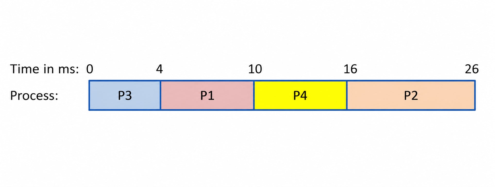
Since P3 has the shortest burst time, it executes first.
After P3 completes, both P1 and P4 have the same burst time (6 ms). Since P1 arrived before P4, it is executed first according to the FCFS rule.
The execution order is:
P3 → P1 → P4 → P2
Average Turnaround Time
Example 2
Now consider processes arriving at different times.
| Process | Arrival Time | Burst Time |
|---|---|---|
| P1 | 0 | 6 |
| P2 | 4 | 10 |
| P3 | 4 | 4 |
| P4 | 8 | 3 |
Solution:
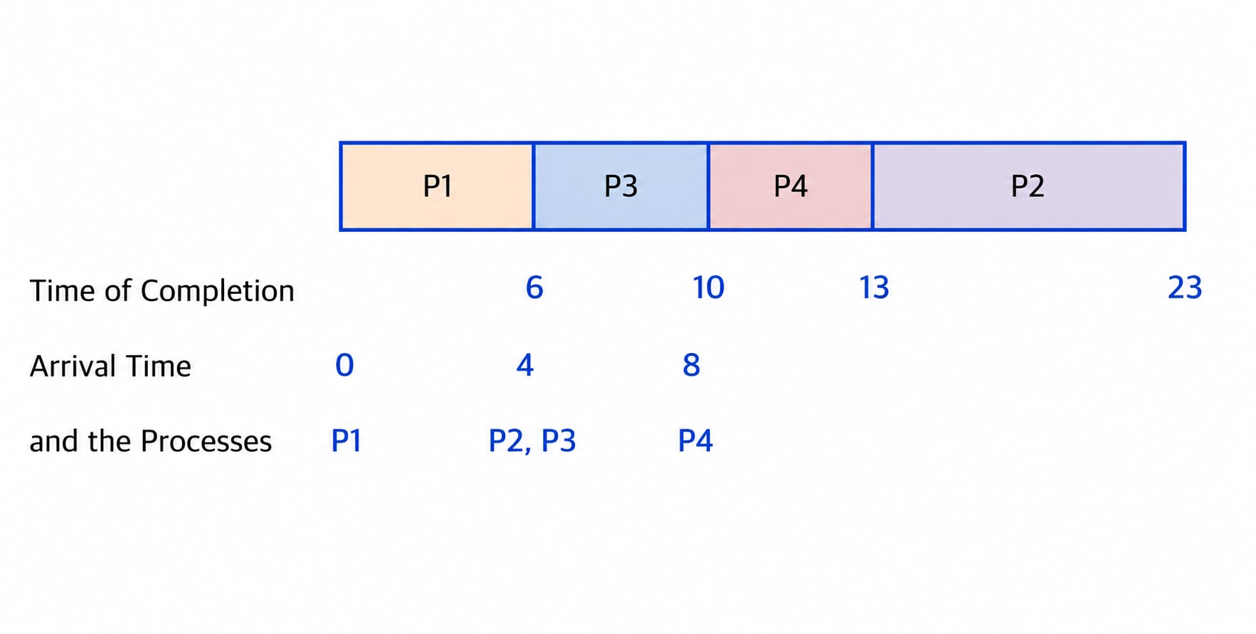
At 0 ms, only P1 is available, so it starts executing.
When P1 finishes at 6 ms, both P2 and P3 are waiting. Since P3 has the shorter burst time, it is selected.
After P3 completes at 10 ms, P4 has already arrived. Between P2 and P4, P4 has the shorter burst time, so it executes next.
The execution order becomes:
P1 → P3 → P4 → P2
Turnaround Time is calculated using:
TAT = CT − AT
- P1: 6 − 0 = 6 ms
- P2: 23 − 4 = 19 ms
- P3: 10 − 4 = 6 ms
- P4: 13 − 8 = 5 ms
Average Turnaround Time
Waiting Time
For Non-Preemptive SJF:
WT = Time when CPU is allocated − Arrival Time
- P1: 0 − 0 = 0 ms
- P2: 13 − 4 = 9 ms
- P3: 6 − 4 = 2 ms
- P4: 10 − 8 = 2 ms
Average Waiting Time
Example of Preemptive SJF (SRTF)
Consider the following processes:
| Process | Arrival Time | Burst Time |
|---|---|---|
| P1 | 0 | 8 |
| P2 | 4 | 10 |
| P3 | 4 | 3 |
| P4 | 10 | 4 |
Solution:
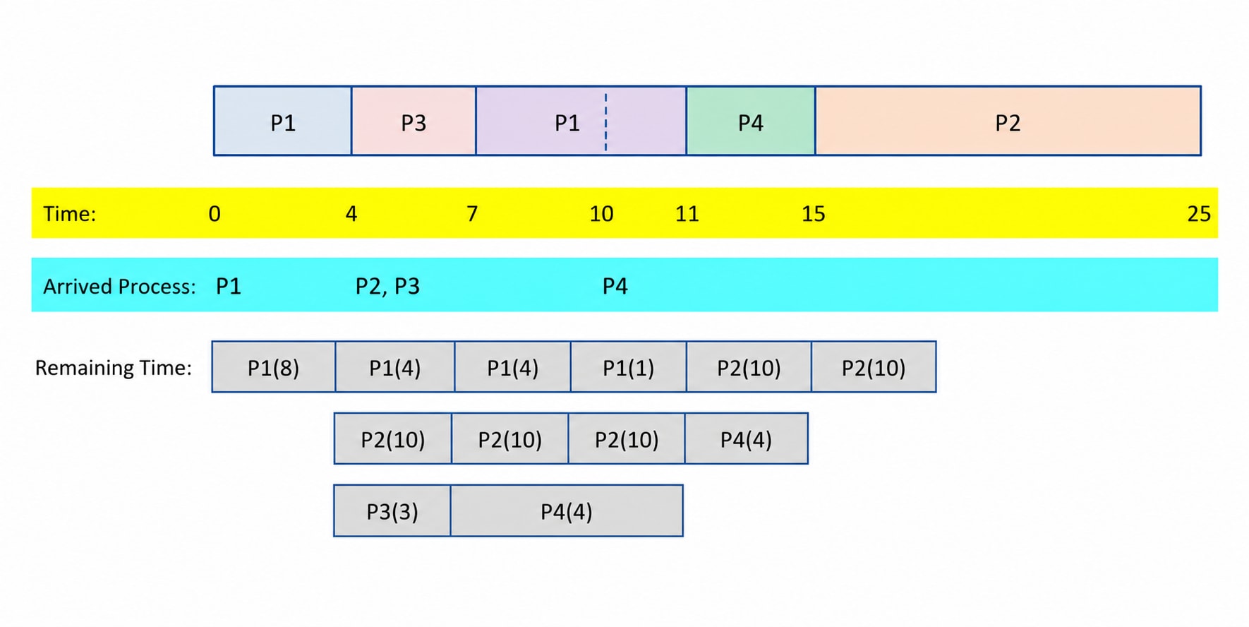
Since SRTF is a preemptive scheduling algorithm, the scheduler checks the remaining execution time whenever:
- A new process arrives.
- A running process completes.
Initially, only P1 is available, so it starts executing.
At 4 ms, P2 and P3 arrive. The remaining execution times are:
- P1 = 4 ms
- P2 = 10 ms
- P3 = 3 ms
Since P3 has the shortest remaining time, P1 is preempted, and P3 starts executing.
After P3 finishes at 7 ms, the scheduler compares the remaining burst times again. P1 now has the shortest remaining time, so it resumes execution.
At 10 ms, P4 arrives. The scheduler again compares the remaining times of all ready processes. Since P1 still has the shortest remaining time, it continues execution without interruption.
The remaining processes execute in the same way until all processes finish.
Average Turnaround Time
Average Waiting Time
Advantages of SJF Scheduling
- SJF significantly reduces the average waiting time compared to FCFS scheduling.
- It improves the average turnaround time.
- It provides better CPU utilization and higher throughput when burst times are estimated accurately.
- It is one of the most efficient scheduling algorithms for minimizing waiting time.
Disadvantages of SJF Scheduling
- Long processes may suffer from starvation if shorter processes continue to arrive.
- In the preemptive version (SRTF), frequent process switching may increase CPU overhead due to repeated context switching.
- Estimating the CPU burst time of a process accurately is difficult. Incorrect estimates can reduce the efficiency of the scheduling algorithm.
- SJF is not suitable when the burst time of processes is unknown in advance.
Note: The performance of the SJF algorithm depends heavily on accurate burst time estimation. If the estimated burst times are incorrect, the scheduling decisions may become inefficient, leading to increased waiting and turnaround times.
3. Priority Non-Preemptive Scheduling
In Non-Preemptive Priority Scheduling, once a process is assigned to the CPU, it continues executing until it finishes. Even if a higher-priority process arrives during execution, it must wait until the currently running process completes.
The scheduler selects the highest-priority process only when:
- The currently running process finishes.
- The CPU becomes idle.
This method has fewer context switches because processes are never interrupted during execution.
Features of Non-Preemptive Priority Scheduling
- It is a non-preemptive scheduling algorithm.
- Once a process starts executing, it cannot be interrupted.
- The process with the highest priority is selected whenever the CPU becomes free.
- If multiple processes have the same priority, the FCFS rule is used.
- It has lower context-switching overhead than the preemptive version.
- Long-running processes can increase the waiting time of other processes.
Example 1
Suppose all processes arrive at the same time.
| Process | Burst Time (ms) | Priority |
|---|---|---|
| P1 | 6 | 2 |
| P2 | 10 | 1 |
| P3 | 4 | 3 |
| P4 | 6 | 2 |
Assume that a lower priority number indicates a higher priority.
Solution:
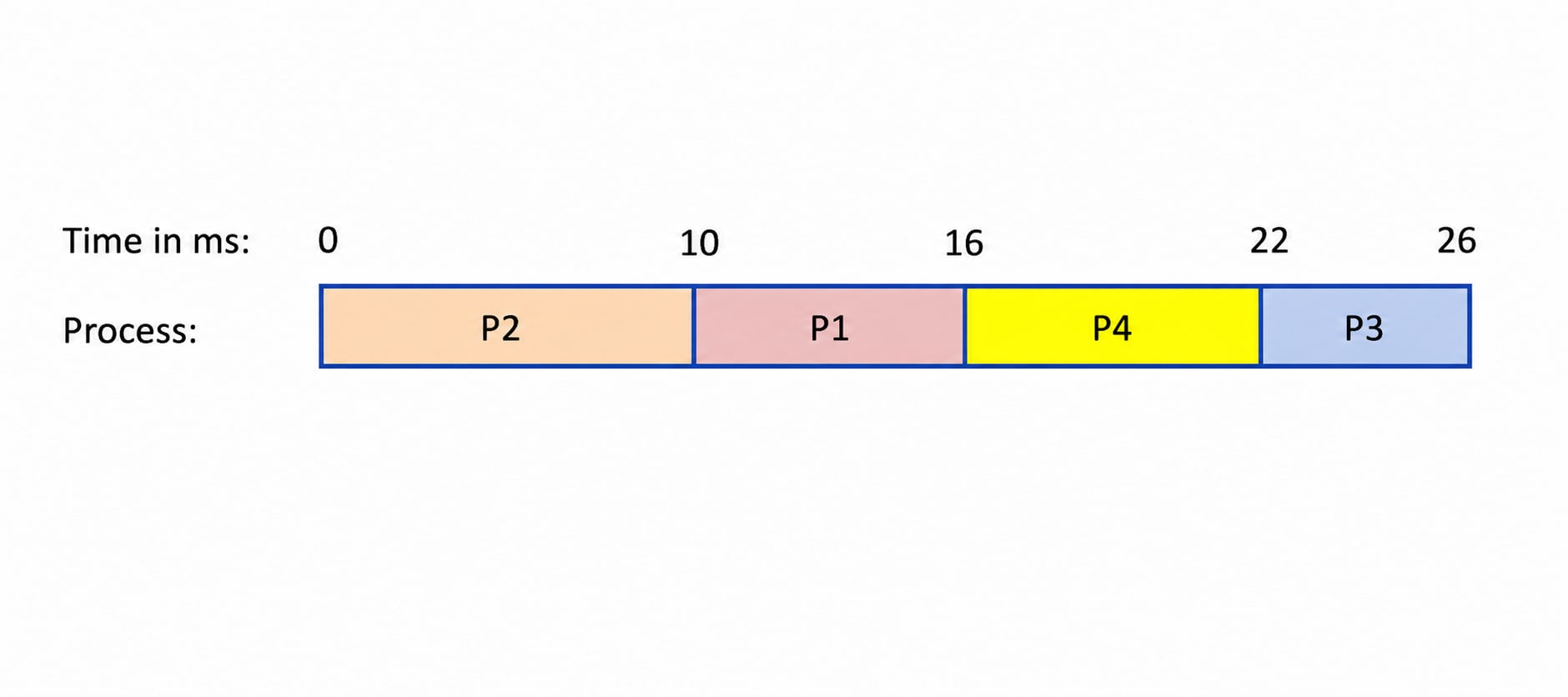
Since P2 has the highest priority (Priority = 1), it executes first. Next, P1 and P4 have the same priority (Priority = 2). According to the FCFS rule, P1 executes before P4 because it arrived first. Finally, P3 executes.
The execution order is:
Average Turnaround Time
Average Waiting Time
Example 2
Now consider processes arriving at different times.
| Process | Arrival Time | Burst Time | Priority |
|---|---|---|---|
| P1 | 0 | 6 | 2 |
| P2 | 4 | 10 | 1 |
| P3 | 4 | 4 | 2 |
| P4 | 8 | 3 | 1 |
Assume that a lower priority value indicates a higher priority.
Solution:
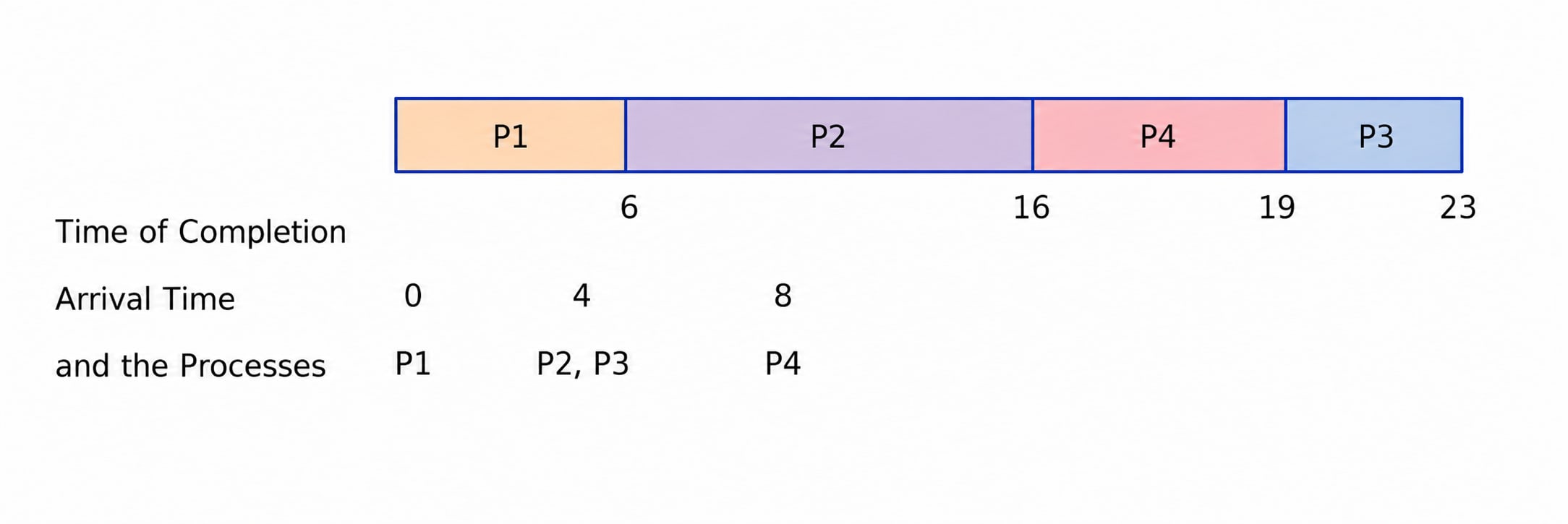
At 0 ms, only P1 is available, so it starts executing. When P1 finishes at 6 ms, both P2 and P3 are waiting. Since P2 has the higher priority, it is selected. After P2 finishes, P4 has already arrived and also has the highest priority, so it executes next. Finally, P3 executes.
The execution order is:
Turnaround Time
P1: 6 − 0 = 6 ms
P2: 16 − 4 = 12 ms
P3: 23 − 4 = 19 ms
P4: 19 − 8 = 11 ms
Average Turnaround Time
Waiting Time
P1: 0 − 0 = 0 ms
P2: 6 − 4 = 2 ms
P3: 19 − 4 = 15 ms
P4: 16 − 8 = 8 ms
Average Waiting Time
4. Highest Response Ratio Next (HRRN) Scheduling
Highest Response Ratio Next (HRRN) is a non-preemptive CPU scheduling algorithm that selects the next process based on its Response Ratio (RR). The response ratio is calculated using the following formula:
Response Ratio (RR)
RR = (Waiting Time + Burst Time) / Burst Timeor
RR = (W + S) / SWhere:
- W = Waiting Time
- S = Burst Time (Service Time)
Whenever the CPU becomes available, the scheduler calculates the response ratio of all processes in the ready queue. The process with the highest response ratio is selected for execution. Since HRRN is a non-preemptive scheduling algorithm, once a process gets the CPU, it continues executing until it finishes.
Features of HRRN Scheduling
- HRRN is a non-preemptive scheduling algorithm.
- The CPU is assigned to the process with the highest response ratio.
- It gives preference to both short processes and processes that have waited longer.
- It is an improved version of the Shortest Job First (SJF) algorithm because it reduces the chances of starvation.
- The scheduler is invoked only when the currently running process finishes or when the ready queue becomes empty.
- It requires fewer context switches than preemptive scheduling algorithms.
Working Principle of HRRN Scheduling
- When the CPU is idle, the first available process is selected for execution.
- After the running process finishes, the scheduler calculates the response ratio of every process waiting in the ready queue.
- The process with the highest response ratio is assigned to the CPU.
- This process runs until completion because HRRN is non-preemptive.
- Steps 2–4 are repeated until all processes have completed execution.
Example of HRRN Scheduling
Consider the following processes.
| Process | Arrival Time | Burst Time |
|---|---|---|
| P1 | 0 | 6 |
| P2 | 4 | 10 |
| P3 | 4 | 4 |
| P4 | 8 | 5 |
Solution:
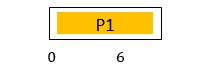
At Time = 0 ms Only P1 is available, so it starts executing immediately. P1 completes at 6 ms.
At Time = 6 ms P1 has completed execution. The processes waiting in the ready queue are P2 and P3.
Response Ratio of P2
RR = (W + S) / S

= (2 + 10) / 10

= 1.2
Response Ratio of P3
RR = (2 + 4) / 4

= 1.5
Since P3 has the higher response ratio, it is selected for execution.
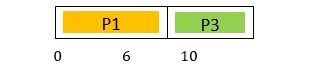
At Time = 10 ms P3 completes execution. The processes waiting are P2 and P4.
Response Ratio of P2
RR = (6 + 10) / 10

= 1.6
Response Ratio of P4
RR = (2 + 5) / 5

= 1.4
Since P2 has the higher response ratio, it is selected.

At Time = 20 ms P2 completes execution. Only P4 remains in the ready queue, so it is assigned to the CPU immediately.
The final execution order is:

Turnaround Time
- P1: 6 − 0 = 6 ms
- P2: 20 − 4 = 16 ms
- P3: 10 − 4 = 6 ms
- P4: 25 − 8 = 17 ms
Average Turnaround Time
Waiting Time
- P1: 0 − 0 = 0 ms
- P2: 10 − 4 = 6 ms
- P3: 6 − 4 = 2 ms
- P4: 20 − 8 = 12 ms
Average Waiting Time
Advantages of HRRN Scheduling
- HRRN provides a good balance between short and long processes.
- It reduces the starvation problem found in the Shortest Job First (SJF) algorithm.
- Shorter processes usually receive faster service, improving average waiting and turnaround times.
- Since it is non-preemptive, fewer context switches occur, reducing CPU overhead.
- It provides better fairness than SJF by increasing the priority of processes that wait longer.
Disadvantages of HRRN Scheduling
- HRRN requires the CPU burst time of each process to be known in advance.
- Estimating burst time accurately is difficult in real systems.
- The scheduler must calculate the response ratio for every waiting process whenever the CPU becomes free, increasing scheduling overhead.
- HRRN does not support process priorities. Therefore, an important process may still have to wait if its response ratio is lower than that of other processes.
- It is less suitable for real-time systems where priority-based scheduling is required.
Note: HRRN is considered an improved version of Shortest Job First (SJF) because it not only considers the burst time of a process but also its waiting time. As a process waits longer in the ready queue, its response ratio increases, reducing the chances of starvation and making the scheduling process fairer.
2. Preemptive Scheduling
In Preemptive Scheduling, the operating system gives the CPU to a process for a fixed amount of time, called a time slice or time quantum. When the allotted time is over, or if a higher-priority process arrives, the operating system can interrupt the currently running process and give the CPU to another process.
The interrupted process is moved from the Running state to the Ready state so that it can continue executing later. If a higher-priority process becomes ready, the operating system immediately assigns the CPU to that process. Preemptive scheduling improves system responsiveness because important or interactive processes do not have to wait for a long-running process to finish.
Advantages
- Better response time.
- High-priority processes get CPU quickly.
- Improves CPU utilization.
- Suitable for modern multitasking operating systems.
Disadvantages
- More context switching.
- Higher overhead due to frequent CPU switching.
- More complex to implement.
Preemptive Scheduling Algorithms
1. Round Robin (RR) Scheduling
Round Robin (RR) is a CPU scheduling algorithm in which each process is assigned a fixed amount of CPU time, called the time quantum or time slice. Processes are executed one after another in a circular order, ensuring that every process gets an equal opportunity to use the CPU. If a process completes its execution within its assigned time quantum, it leaves the system. Otherwise, it is preempted, moved to the end of the ready queue, and waits for its next turn. The ready queue follows the First Come, First Served (FCFS) order.
Round Robin is a preemptive scheduling algorithm because the CPU can interrupt a running process once its time quantum expires, even if the process has not finished execution. It can be considered a preemptive version of the FCFS scheduling algorithm.
Features of Round Robin Scheduling
- RR is a preemptive CPU scheduling algorithm.
- Each process is assigned an equal time quantum for execution.
- Processes are executed in a circular order using the FCFS ready queue.
- A running process is preempted when its time quantum expires.
- It prevents starvation by giving every process a fair chance to execute.
- It is simple to implement and widely used in time-sharing operating systems.
- The performance of RR scheduling depends heavily on the selected time quantum.
Working Principle of Round Robin Scheduling
- Every new process is added to the end of the ready queue following the FCFS principle.
- The process at the front of the queue is assigned to the CPU.
- If the process finishes before or exactly at the end of its time quantum, it leaves the system, and the next process gets the CPU.
- If the process does not finish within its time quantum, it is preempted, its remaining burst time is saved, and it is moved to the end of the ready queue.
- A context switch occurs, and the next process in the queue starts execution.
- These steps continue until all processes have completed their execution.
Example of Round Robin Scheduling
Consider the following processes, all arriving at the same time.
| Process | Burst Time (ms) |
|---|---|
| P1 | 8 |
| P2 | 10 |
| P3 | 6 |
| P4 | 4 |
Assume the time quantum is 2 ms. Draw the Gantt Chart and calculate the Average Turnaround Time and Average Waiting Time.
GANTT Chart with time quantum of 2ms:
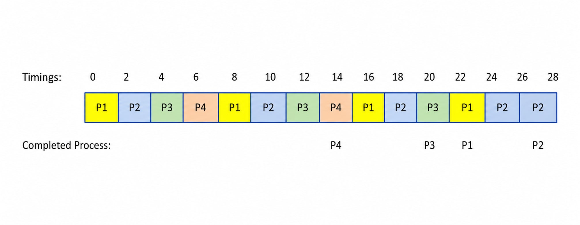
Average Turnaround Time
Average Waiting Time - The waiting time of each process is obtained by multiplying the number of waiting time slices by the time quantum.
Average WT
Advantages of Round Robin Scheduling
- Every process receives an equal share of CPU time, making the algorithm fair.
- Starvation is avoided because each process gets a chance to execute after every time quantum.
- It does not require prior knowledge of the CPU burst time of processes.
- It is simple to understand and easy to implement.
- It is widely used in time-sharing operating systems because it provides better response time.
- Unlike FCFS, the convoy effect is greatly reduced.
Disadvantages of Round Robin Scheduling
- The performance of RR scheduling depends heavily on the selected time quantum.
- If the time quantum is too large, RR behaves similarly to FCFS, resulting in poor response time.
- If the time quantum is too small, the CPU spends more time performing context switches than executing processes, reducing overall system performance.
- Frequent context switching increases CPU overhead.
- RR does not consider process priority, so high-priority and low-priority processes receive the same amount of CPU time, which may reduce system efficiency in priority-based environments.
Note: Choosing an appropriate time quantum is crucial. A very small time quantum increases context-switching overhead, while a very large time quantum makes Round Robin behave like FCFS. An optimal time quantum provides a good balance between response time and CPU utilization.
2. Priority Preemptive Scheduling
In Preemptive Priority Scheduling, the CPU is always assigned to the highest-priority process. If a new process with a higher priority arrives while another process is executing, the currently running process is immediately interrupted and moved back to the ready queue. The new higher-priority process then starts execution. This scheduling method provides faster response for important processes but increases the number of context switches.
Features of Preemptive Priority Scheduling
- It is a preemptive scheduling algorithm.
- A running process can be interrupted by a newly arrived higher-priority process.
- The CPU always executes the highest-priority process available.
- If two processes have the same priority, FCFS is used.
- It provides quick response to high-priority processes.
- It involves more context switching than the non-preemptive version.
Example
Consider the following processes.
| Process | Arrival Time | Burst Time | Priority |
|---|---|---|---|
| P1 | 0 | 8 | 3 |
| P2 | 4 | 10 | 2 |
| P3 | 4 | 3 | 3 |
| P4 | 10 | 4 | 1 |
Assume that a lower priority value indicates a higher priority.
Solution:
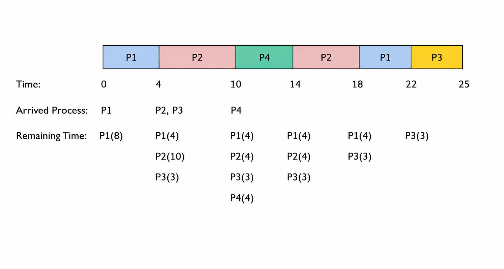
Initially, only P1 is available, so it starts executing. At 4 ms, P2 and P3 arrive. Since P2 has a higher priority than P1, it immediately preempts P1. At 10 ms, P4 arrives with the highest priority and preempts P2. After P4 finishes, the scheduler selects the highest-priority process among the remaining processes. P2 continues execution because it has a higher priority than P1 and P3. When P2 completes, P1 and P3 have the same priority. Therefore, P1 executes first because it arrived earlier. Finally, P3 executes.
The execution order is:
Average Turnaround Time
Average Waiting Time
Process Scheduling Queues
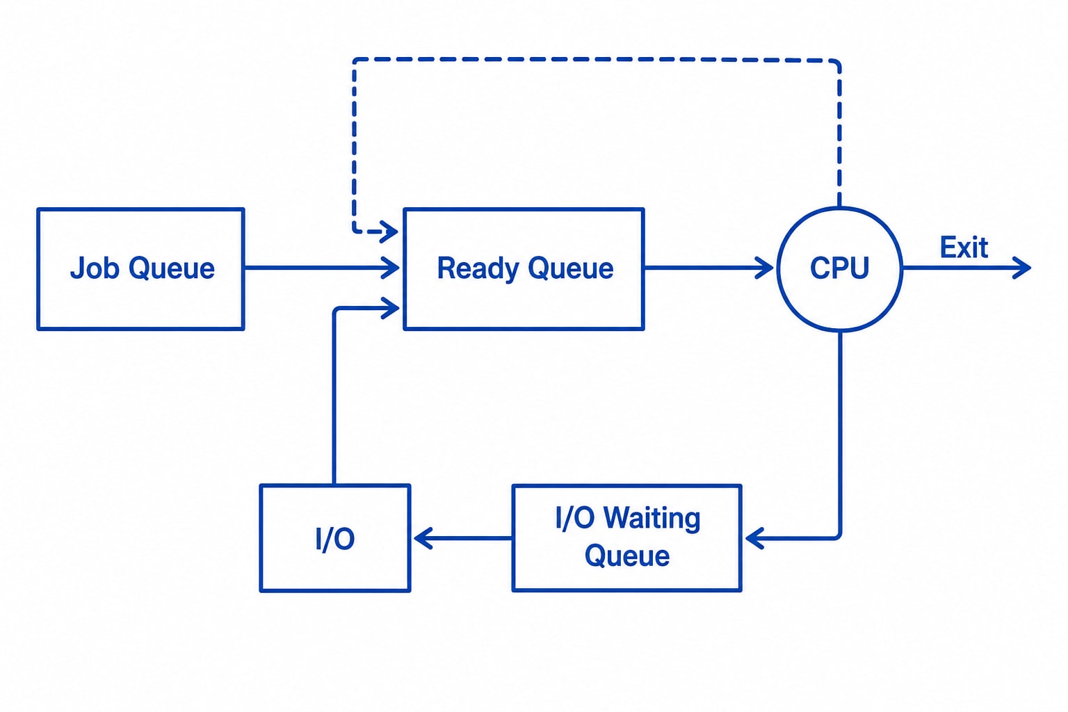
The operating system manages all processes using Process Control Blocks (PCBs). Every process has its own PCB, which stores important information about that process. To organize processes efficiently, the operating system places PCBs into different process scheduling queues. Each process state has its own queue. Whenever the state of a process changes, its PCB is removed from the current queue and placed into the appropriate new queue.
For example, if a process changes from the Ready state to the Running state, its PCB is removed from the Ready Queue and placed into the Running state. The operating system mainly maintains the following scheduling queues.
-
Job Queue - The Job Queue contains all the processes present in the system. Every new process enters this queue when it is created. From here, the operating system decides which processes should be loaded into memory.
-
Ready Queue - The Ready Queue contains all the processes that are already loaded into the main memory and are ready to execute. These processes are only waiting for the CPU to become available. Whenever the CPU becomes free, the CPU scheduler selects one process from the Ready Queue and assigns the CPU to it. Every newly created process is first placed in the Ready Queue after it is admitted into memory.
-
Device Queue - The Device Queue contains processes that are waiting for an Input/Output (I/O) device, such as a keyboard, printer, hard disk, or network device. If a process requests an I/O operation and the required device is busy, the process cannot continue execution. It is moved to the Device Queue and waits until the device becomes available.
After the I/O operation is completed, the process is moved back to the Ready Queue.
Process Scheduling Queuing
The operating system can use different scheduling algorithms to manage these queues. Some common scheduling policies are:
- FIFO (First In First Out)
- Round Robin (RR)
- Priority Scheduling
The Operating System Scheduler decides how processes move between different queues, especially between the Ready Queue and the Running state.
Since each CPU core can execute only one process at a time, only one process is allowed to use a CPU core at any given moment. The scheduler continuously selects the next suitable process according to the scheduling algorithm being used.
Two-State Process Model
The Two-State Process Model is the simplest process model. In this model, a process can exist in only two states:
-
Running - A process is in the Running state when the CPU is executing its instructions.Whenever the operating system selects a process from the Ready Queue and assigns the CPU to it, the process enters the Running state. Only one process can be in the Running state on a single CPU core at any given time.
-
Not Running - A process is in the Not Running state when it is not currently using the CPU. These processes wait in a queue until the CPU becomes available. Each process in the queue is represented by a pointer, and the queue is generally implemented using a linked list. The Dispatcher is responsible for selecting a process from this queue and assigning it to the CPU. If a running process is interrupted, it is moved back to the waiting queue. If the process completes its execution or is terminated, it is removed from the system. After that, the dispatcher selects another process from the queue and starts its execution.
Schedulers
Schedulers are special system software which handle process scheduling in various ways. Their main task is to select the jobs to be submitted into the system and to decide which process to run
Its main responsibility is to decide:
- Which processes should enter the system.
- Which process should be loaded into memory.
- Which process should get the CPU.
- Which process should be temporarily removed from memory.
The operating system mainly uses three types of schedulers:
- Long-Term Scheduler
- Short-Term Scheduler
- Medium-Term Scheduler
The Long-Term Scheduler is also called the Job Scheduler. Its main job is to select processes from the Job Queue and load them into the main memory so that they can be executed by the CPU. The Long-Term Scheduler controls the degree of multiprogramming, which means it controls how many processes remain in memory at the same time.
Its goal is to maintain a proper balance between:
- CPU-bound processes, which spend most of their time using the CPU.
- I/O-bound processes, which spend most of their time waiting for input or output operations.
A good balance helps improve overall system performance. If the number of incoming processes is almost equal to the number of completed processes, the degree of multiprogramming remains stable. Modern time-sharing operating systems usually have very little or no Long-Term Scheduler because processes are admitted into memory quickly. Whenever a process changes from the New state to the Ready state, the Long-Term Scheduler performs this task.
The Short-Term Scheduler is also called the CPU Scheduler. Its main responsibility is to select one process from the Ready Queue and assign the CPU to it. Whenever the CPU becomes free, the Short-Term Scheduler immediately selects the next process for execution.
It changes the process state from Ready to Running. Since this scheduler runs very frequently, it must make decisions very quickly. Therefore, it is the fastest scheduler in the operating system. The Short-Term Scheduler is also known as the Dispatcher because it dispatches the selected process to the CPU.
The Medium-Term Scheduler manages the swapping process. Sometimes the main memory becomes full or the operating system wants to reduce the number of processes currently in memory. In such cases, the Medium-Term Scheduler temporarily removes some processes from memory and stores them in secondary storage (hard disk or SSD).
This process is called Swapping, and the process is said to be swapped out or rolled out. Later, when enough memory becomes available, the scheduler brings the process back into the main memory. This is called swapping in or rolling in.
The Medium-Term Scheduler helps:
- Free main memory.
- Reduce the degree of multiprogramming.
- Improve overall system performance.
Comparison of Schedulers
| Long-Term Scheduler | Short-Term Scheduler | Medium-Term Scheduler |
|---|---|---|
| Also called the Job Scheduler. | Also called the CPU Scheduler or Dispatcher. | Also called the Swapping Scheduler. |
| Slower than the Short-Term Scheduler. | Fastest among all schedulers. | Faster than Long-Term but slower than Short-Term Scheduler. |
| Controls the degree of multiprogramming. | Has very little control over the degree of multiprogramming. | Reduces the degree of multiprogramming by swapping processes. |
| Usually absent or minimal in time-sharing systems. | Always active in time-sharing systems. | Used whenever swapping is required. |
| Selects processes from the Job Queue and loads them into memory. | Selects a ready process and gives it the CPU. | Removes and later reloads processes into memory. |
Context Switching
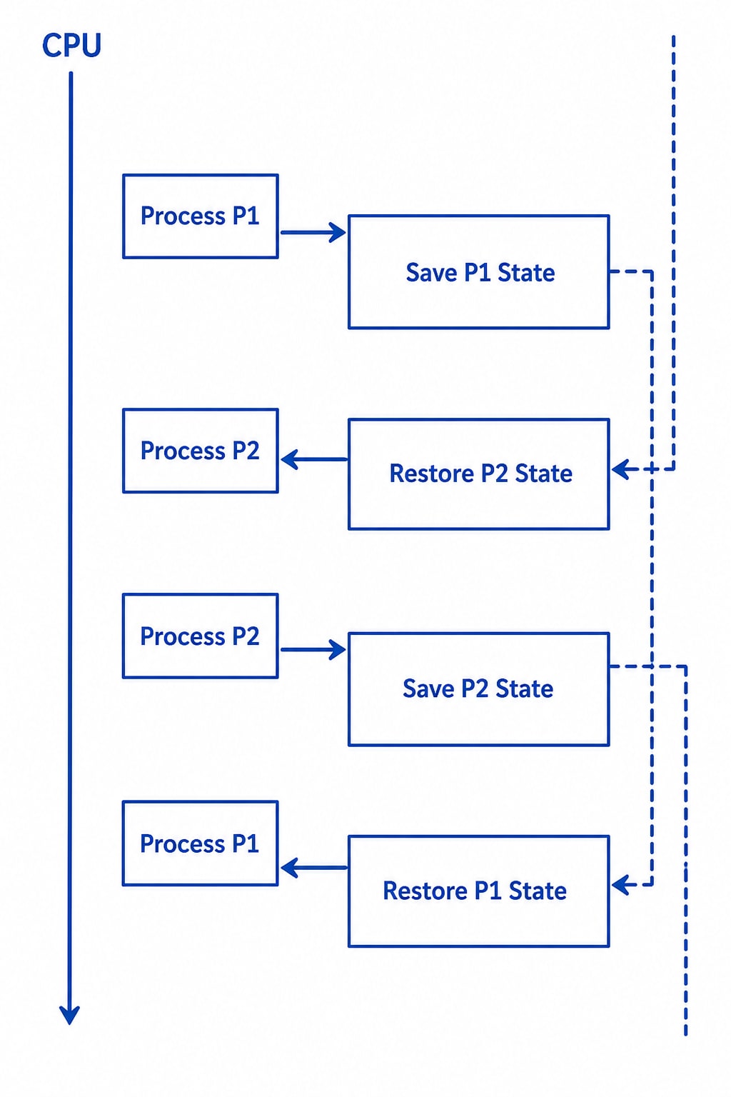
Context Switching is the process of saving the current state of one process and restoring the state of another process so that multiple processes can share a single CPU.
Whenever the operating system switches the CPU from one process to another, it first saves the current process's information in its Process Control Block (PCB). Later, when that process gets the CPU again, its saved information is restored, allowing it to continue execution from exactly where it stopped. Context switching is an important feature of multitasking operating systems because it allows multiple processes to run smoothly even though only one process uses the CPU at a time.
When the scheduler decides to switch the CPU from one process to another, the following steps take place:
- The operating system saves the current state of the running process into its PCB.
- The scheduler selects the next process from the Ready Queue.
- The operating system loads the saved state of the selected process from its PCB.
- The Program Counter, CPU registers, and other information are restored.
- The new process continues execution from the exact instruction where it was previously interrupted.
During a context switch, the operating system stores the following information:
- Program Counter (PC): Stores the address of the next instruction to be executed.
- Scheduling Information: Stores process priority and other scheduling details.
- Base and Limit Register Values: Store information related to the memory allocated to the process.
- CPU Registers: Store the current values of all CPU registers.
- Process State: Stores whether the process is Running, Ready, Waiting, or Terminated.
- I/O State Information: Stores information about the input/output operations being performed.
- Accounting Information: Stores CPU usage, execution time, process statistics, and other accounting details.
Although context switching is necessary for multitasking, it also takes CPU time because the operating system has to save and restore process information. Therefore, frequent context switching increases system overhead and can slightly reduce overall performance.
Operations on Processes
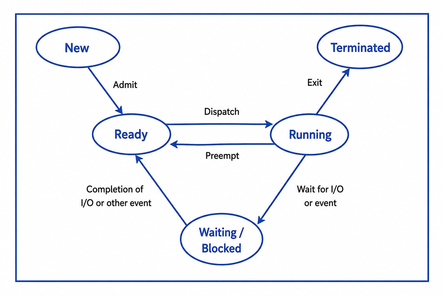
A process is a program in execution that undergoes a number of states in its lifetime. In each of these states, a process undergoes certain operations that enable the process to execute into completion.
States of a Process
A process does not remain in the same state throughout its lifetime. As it executes, it moves from one state to another depending on what it is doing. The main states of a process are explained below.
1. New – This is the first state of a process. In this state, the operating system creates the process. The process has been created successfully, but it has not started executing yet.
2. Ready – In the Ready state, the process has all the resources required for execution except the CPU. It is loaded into the main memory and is ready to run, but it must wait until the CPU scheduler assigns the CPU to it.
3. Running – A process enters the Running state when the CPU is assigned to it. In this state, the CPU executes the instructions of the process. The process continues running until it completes its execution, is interrupted, or moves to another state.
4. Waiting (Blocked) – A process enters the Waiting state when it cannot continue its execution until a particular event occurs. For example, it may be waiting for an input/output (I/O) operation to finish, waiting for user input, or waiting for another resource. During this state, the process does not use the CPU. Once the required event is completed, the process moves back to the Ready state.
5. Terminated (Exit) – This is the final state of a process. A process enters this state after it completes its execution or when it is terminated by the operating system. After termination, all the resources used by the process are released, and the process is removed from the system.
Different Process Operations
During its lifetime, a process performs different operations. These operations take place when the process is in a particular state or when it moves from one state to another. Each operation helps the operating system manage the process efficiently.
The main operations performed on a process are:
Process Creation
Process Dispatch
Process Pre-emption
Process Blocking
Process Termination
Process Creation
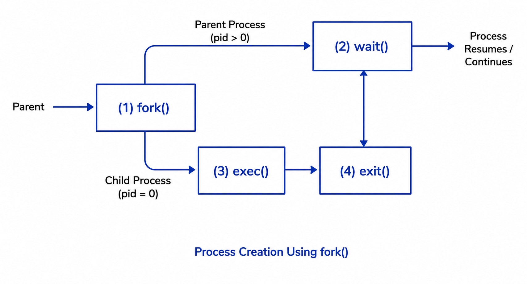
Process Creation is the first operation that takes place when a process enters the system. During this operation, the operating system creates a new process and prepares it for execution. Process creation is related to the New state of a process.
A process can be created for several reasons, which are explained below.
1. System Initialization – When the computer starts, the operating system automatically creates several system processes and background processes that are necessary for the system to work properly. These processes help manage system resources and perform important background tasks.
2. User Request – A user can create a process by starting a program. For example, when a user opens a web browser, media player, or text editor, the operating system creates a new process to run that program.
3. Child Process System Call – A process that is already running can create another process by using a process creation system call, such as fork() in UNIX-based operating systems.
The process that creates the new process is called the Parent Process, and the newly created process is called the Child Process.
A child process can have only one parent process, but a parent process can create many child processes.
At the beginning, both the parent and child processes have the same program code, open files, and environment variables. However, they have different address spaces (memory spaces), which means each process executes independently and does not directly affect the memory of the other process.
4. Batch System – In a batch processing system, the operating system automatically creates processes to execute batch jobs. These jobs are processed one after another without requiring direct interaction from the user.
After a process is created successfully, it is loaded into memory and enters the Ready state, where it waits for the CPU scheduler to assign the CPU. Once the CPU is assigned, the process moves to the Running state and begins executing its instructions.
Process Dispatch
Process Dispatch is the operation in which a process in the Ready state is selected by the CPU scheduler and given the CPU for execution. When the scheduler chooses a process according to the scheduling algorithm, the dispatcher assigns the CPU to that process so it can start running.
Process dispatch can happen in the following situations:
1. CPU Becomes Idle – When the CPU finishes executing the current process and becomes free, the scheduler selects another process from the Ready Queue and dispatches it to the CPU.
2. Ready Queue Contains Processes – If there are one or more processes waiting in the Ready Queue, the scheduler selects one of them and assigns it to the CPU.
3. Time Quantum Expires – In preemptive scheduling, each process is given a fixed amount of CPU time called a time quantum. When this time expires, the scheduler may stop the current process and dispatch another ready process.
4. A Higher-Priority Process Arrives – If a new process with a higher priority enters the Ready Queue, the scheduler may immediately assign the CPU to that process.
5. Hardware Interrupt Occurs – A hardware interrupt, such as input from a keyboard or the completion of an I/O operation, may cause the scheduler to dispatch another process.
When a new process is selected for execution, the operating system loads the process information stored in its Process Control Block (PCB). This information includes the Program Counter, CPU registers, scheduling information, and other details required for execution. After loading this information, the selected process starts running on the CPU.
Process Pre-emption
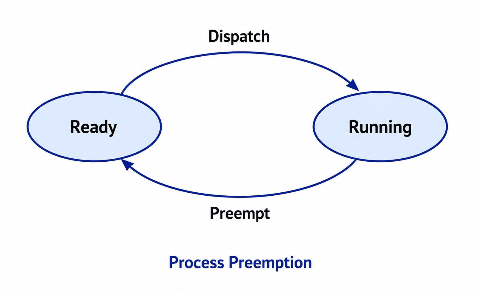
Process Pre-emption is the operation in which the operating system temporarily stops the execution of the currently running process and gives the CPU to another process. Pre-emption is mainly used in preemptive scheduling, where the operating system can interrupt a running process whenever required.
Process pre-emption may occur in the following situations:
1. Time Quantum Expires – When the time allocated to the running process is over, the operating system interrupts it and gives the CPU to another process.
2. Higher-Priority Process Enters the Ready Queue – If a process with a higher priority becomes ready, the operating system may stop the current process and assign the CPU to the higher-priority process.
3. Hardware Interrupt Occurs – A hardware interrupt may require the operating system to stop the current process temporarily and execute another process.
When a process is pre-empted, it does not lose its progress. Before removing it from the CPU, the operating system saves the complete state of the process in its Process Control Block (PCB).
This saved information includes the current Program Counter, CPU registers, scheduling information, memory information, and other important details. Later, when the process gets the CPU again, this information is restored, allowing the process to continue execution from the exact point where it was interrupted.
The process of saving the state of one process and restoring the state of another process is called Context Switching.
Process Blocking
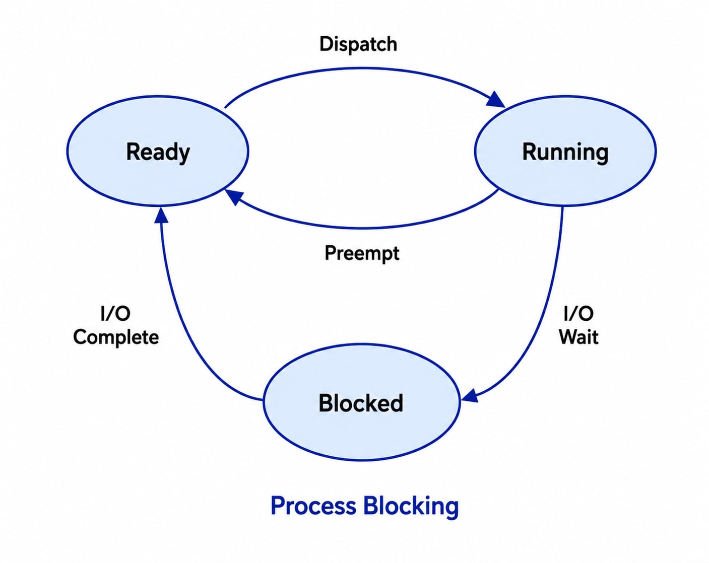
Process Blocking is the operation in which a running process is moved to the Waiting (Blocked) state because it cannot continue its execution until a specific event occurs. A process is blocked only when it needs something before it can continue its work. A process may become blocked for the following reasons:
1. Input/Output (I/O) Request – A process may request an I/O operation, such as reading data from a file, writing data to a disk, or communicating with a printer. Since I/O operations do not require the CPU continuously, the process is moved to the Waiting state until the operation is completed.
2. Waiting for User Input – A process may need input from the user, such as entering text from the keyboard. Until the user provides the required input, the process remains in the Waiting state.
3. Waiting for a Resource – A process may need a resource that is currently being used by another process. It must wait until that resource becomes available.
4. Waiting for Another Event – A process may also wait for another process to finish or for any system event required to continue execution.
When a process enters the Waiting state, the operating system removes it from the CPU and assigns the CPU to another ready process. This ensures that the CPU does not remain idle. Once the required event is completed, the operating system moves the blocked process back to the Ready state. The process then waits for the CPU scheduler to assign the CPU again.
Process Termination
Process Termination is the operation in which a process finishes its execution and is removed from the system. During process termination, the operating system releases all the resources that were allocated to the process, such as memory, files, I/O devices, and other system resources. After termination, the process no longer exists in the system.
A process may be terminated for several reasons.
1. Normal Completion of Execution – This is the most common reason for process termination. When a process successfully executes its last instruction, the operating system automatically terminates it and releases all its allocated resources.
2. Parent Process Terminates the Child Process – A parent process may terminate one of its child processes if the child process is no longer required.
Before terminating, the child process sends its status information to the parent process. If the parent process itself is terminated, all of its child processes are also terminated because they cannot continue running without their parent.
3. Operating System Errors – The operating system may terminate a process if it detects serious service errors or illegal operations that prevent the process from continuing safely.
4. Hardware Failure – Hardware problems, such as memory failure, disk failure, or other hardware malfunctions, may also cause a process to terminate unexpectedly.
Steps Involved in Process Termination
In most cases, a process is terminated after it completes its execution. The following steps take place during the termination process.
1. Sending the SIGTERM Signal – The parent process sends a SIGTERM (Terminate Signal) to the child process to inform it that it should terminate.
2. Cleanup Operations – After receiving the SIGTERM signal, the child process performs several cleanup tasks before exiting. These tasks include:
- Releasing all allocated memory.
- Closing all open files.
- Releasing shared resources.
- Giving up access to shared variables and system tables.
- Saving any necessary information before exiting.
3. Process Exit – After completing all cleanup operations, the child process exits.
4. Returning Control – Once the child process has exited, control returns to the parent process or the operating system. Finally, all the resources used by the terminated process are completely released and become available for other processes.
Inter-Process Communication
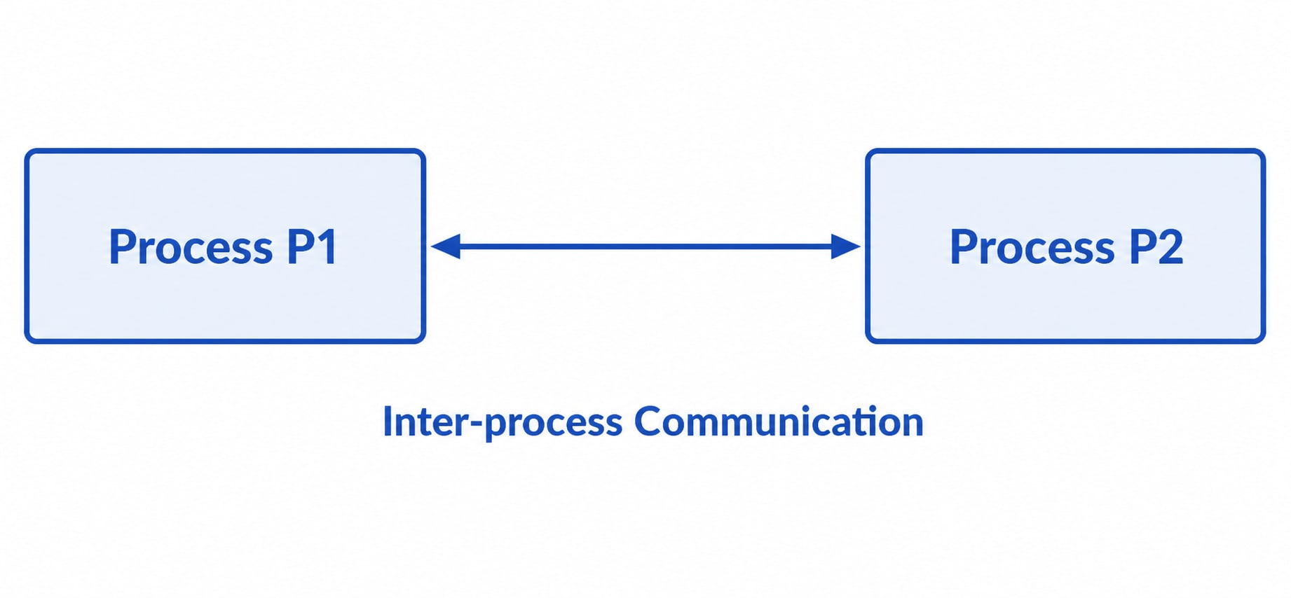
Inter-Process Communication (IPC) is a mechanism that allows two or more processes to communicate and exchange data with each other. It enables processes to share information and system resources without interfering with each other's execution. Using IPC, one process can inform another process that an event has occurred or that some data has been transferred. This allows different processes to work together efficiently while running at the same time.
Inter-Process Communication Importance
Inter-Process Communication (IPC) provides several benefits to an operating system.
- It allows faster communication between processes.
- It supports parallel processing, where multiple processes work at the same time.
- It makes multitasking more efficient by allowing different processes to communicate.
- It allows processes to share memory and system resources without creating unnecessary copies of data, which helps save memory.
- It provides proper synchronization between processes so that they can work together without conflicts.
Types of Processes in IPC
Processes that run at the same time in an operating system can be divided into two categories.
1. Independent Processes – Independent processes do not share any data or resources with other processes. Since they work independently, they cannot affect other processes, and they are not affected by the execution of other processes in the system.
2. Cooperating Processes – Cooperating processes share data, resources, or information with other processes. Because they communicate with each other, one process can affect another process, and it can also be affected by it. These processes need Inter-Process Communication (IPC) to exchange information and coordinate their work properly.
Synchronization in Inter-Process Communication
Synchronization is an important part of Inter-Process Communication. It ensures that multiple processes work together in the correct order without creating conflicts while sharing data or resources. Synchronization can be managed either by the operating system or by the communicating processes themselves.
Some common methods used for synchronization are explained below.
1. Semaphore – A Semaphore is a special variable used to control access to a shared resource when multiple processes want to use it at the same time. It helps prevent conflicts by allowing only the permitted number of processes to access the shared resource.
There are two types of semaphores:
- Binary Semaphore – It has only two values, 0 and 1, and is mainly used for mutual exclusion.
- Counting Semaphore – It can have multiple values and is used when several processes are allowed to access the same resource at the same time.
2. Mutual Exclusion (Mutex) – Mutual Exclusion, also called Mutex, ensures that only one process or thread can enter the Critical Section at a time. The Critical Section is the part of a program where shared data or shared resources are accessed. By allowing only one process to enter the Critical Section, Mutual Exclusion prevents Race Conditions, where multiple processes try to modify the same data at the same time.
3. Barrier – A Barrier is a synchronization method that forces all processes to wait until every process reaches a specific point in the program. No process is allowed to continue until all the participating processes have reached the barrier. Barriers are commonly used in parallel programming to keep all processes synchronized.
4. Spinlock – A Spinlock is a type of lock used to control access to shared resources. If a process tries to acquire a spinlock that is already being used by another process, it continuously checks whether the lock has become available instead of going to sleep. This continuous checking is called Busy Waiting because the process remains active but does not perform any useful work while waiting.
Why is Inter-Process Communication Necessary?
Inter-Process Communication is necessary for several reasons in process management.
1. Information Sharing – Sometimes multiple users or multiple processes need access to the same information. The operating system must provide a way for them to share this information safely. IPC allows different processes to exchange data, send commands, and coordinate their actions so that they can work together without conflicts.
2. Achieving Modularity – Large programs are usually divided into smaller modules to make them easier to develop, test, and maintain. Each module may run as a separate process. Since these processes are working on different parts of the same task, they need to communicate with each other, exchange data, and coordinate their activities. IPC makes this communication possible and helps achieve modularity.
3. Faster Process Execution – Proper communication and synchronization between processes help complete tasks more quickly. A large task can be divided into several smaller subtasks, and each subtask can run in parallel on different processes. IPC allows these parallel processes to exchange information and coordinate their progress. As a result, the overall task is completed faster, improving the performance of the system.
4. Convenience – Modern operating systems allow users to perform many tasks at the same time. For example, a user can edit a document, listen to music, browse the internet, and download files simultaneously.
This convenience is possible because different processes communicate and coordinate with each other using Inter-Process Communication (IPC).
How to Implement Inter-Process Communication (IPC)?
Inter-Process Communication (IPC) can be implemented using two main methods:
1. Shared Memory
2. Message Passing
Both methods allow processes to communicate with each other, but they work in different ways.
1. Shared Memory
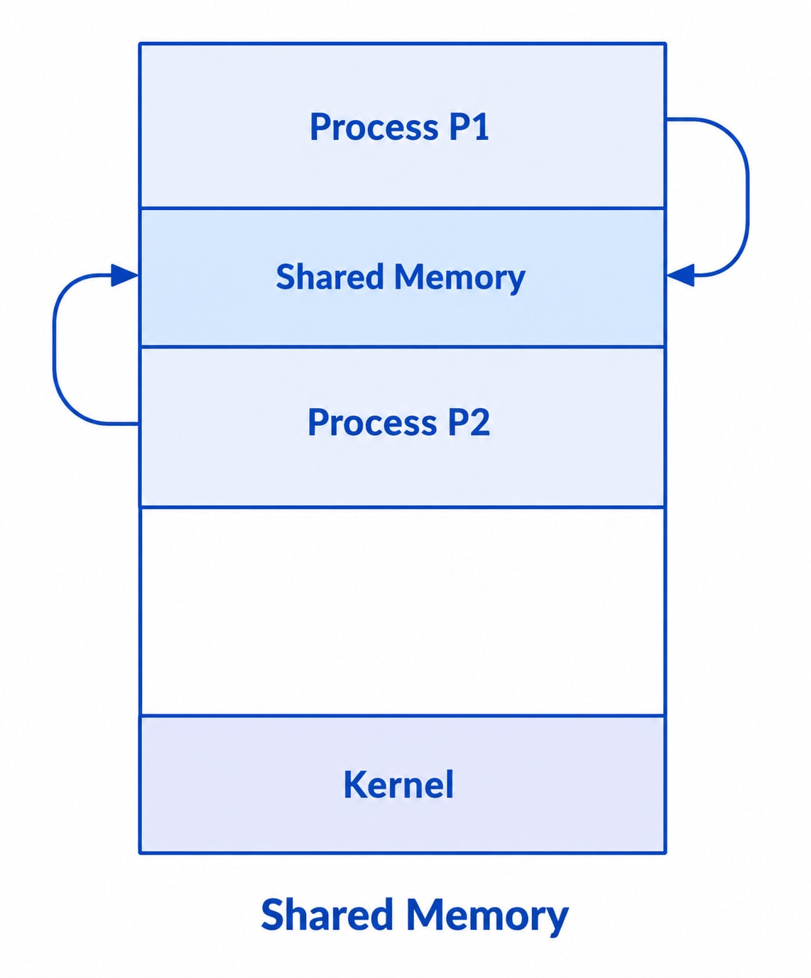
Shared Memory is a method of Inter-Process Communication in which multiple processes can access the same memory area at the same time. Instead of sending data from one process to another, both processes use a common memory region to read and write data. Since the data is stored only once in shared memory, communication becomes faster and more efficient. Shared Memory is supported by most operating systems, including Linux (POSIX systems) and Windows.
How Shared Memory Works
For Shared Memory to work, a shared memory region (also called a common memory area) must first be created. This shared memory region is stored in the address space of the process that creates it. Any other process that wants to communicate using this shared memory must attach the same shared memory region to its own address space. Once both processes are connected to the same shared memory, they can directly read and write data.
Working of Shared Memory
Suppose Process A wants to communicate with Process B.
1. Process A Creates Shared Memory – Process A first creates a shared memory region. This shared memory is stored in the address space of Process A. By creating this common memory area, Process A starts the communication.
2. Process B Connects to Shared Memory – If Process B wants to exchange data with Process A, it must attach the same shared memory region to its own address space. After this step, both processes can access the same memory location.
3. Process A Writes Data – Process A writes data into the shared memory. Since Process B is connected to the same memory region, it can directly read the data without copying it.
4. Process B Updates the Data – If Process B changes or updates the data stored in the shared memory, Process A can immediately see the updated data because both processes are using the same memory area.
In this way, Shared Memory provides fast and efficient communication between processes because the data does not need to be copied from one process to another.
Advantages of Shared Memory
- Communication is very fast because processes access the same memory.
- No extra copy of data is created, which saves memory.
- Suitable for transferring large amounts of data.
- Improves the overall performance of the system.
Disadvantages of Shared Memory
- Proper synchronization is required because multiple processes can access the same memory at the same time.
- If synchronization is not used correctly, problems like Race Conditions and Data Corruption may occur.
- It is more difficult to implement compared to Message Passing.
2. Message Passing
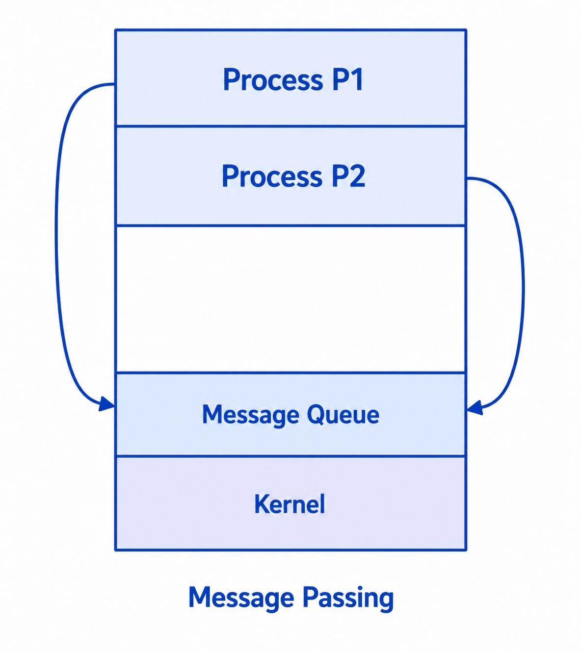
Message Passing is another method of Inter-Process Communication in which processes communicate by sending and receiving messages. In this method, processes do not share the same memory. Instead, one process sends a message, and another process receives it. The message contains the information that needs to be shared. Message Passing is mainly used for exchanging small amounts of data because it avoids conflicts that can occur when multiple processes access the same memory.
How Message Passing Works
In Message Passing, communication takes place through two basic operations:
- Send – One process sends a message.
- Receive – Another process receives the message.
The operating system manages the communication between the processes and ensures that the messages are delivered correctly. Since processes do not share memory, synchronization becomes easier.
Features of Message Passing
- Processes do not need to share the same address space.
- It provides both communication and synchronization between processes.
- It is easier to implement than Shared Memory.
- It is useful in distributed systems, where processes may run on different computers connected through a network.
Ways to Implement Message Passing
Message Passing can be implemented using several communication methods.
1. Pipes - A Pipe is a communication channel used to transfer data between processes. A pipe is unidirectional, which means data can travel in only one direction. If two-way communication is required, two separate pipes are used. Pipes use the standard input and output mechanism for communication and are supported by most operating systems, including Linux (POSIX systems) and Windows.
2. Sockets - A Socket is one endpoint of a communication channel used for sending and receiving data. A Socket is one endpoint of a communication channel used for sending and receiving data.
Sockets can be used for communication:
- Between processes running on the same computer.
- Between processes running on different computers connected through a network. Most modern operating systems use sockets for network communication and Inter-Process Communication.
3. Files - A File is another method of communication between processes. One process can write data into a file, and another process can read the same file whenever required. Since files are stored permanently on storage devices such as hard disks or SSDs, they are commonly used for sharing data between different processes. Almost every operating system supports file-based communication.
4. Signals - A Signal is a special system message sent from one process to another. Signals are generally not used to transfer data. Instead, they are used to notify another process that a particular event has occurred or to request a specific action. For example, signals can be used to stop, continue, or terminate a process. Therefore, signals are mainly used for process control rather than data communication.
5.Message Queue - A Message Queue is a communication mechanism in which messages are stored inside a queue until the receiving process reads them. Processes do not need to be directly connected to communicate through a message queue. One process writes messages into the queue, and another process reads those messages whenever it is ready. Since messages remain in the queue until they are received, Message Queues provide reliable communication between processes. Most modern operating systems support Message Queues for Inter-Process Communication.