Sequential Searching

Sequential searching, also known as linear searching, is a simple algorithm used to find a specific element within a list or array by sequentially examining each element until a match is found or the entire list has been traversed. It's particularly useful when the list is unordered or small.

1. Starting Point: The search begins at the first element of the list.
2. Sequential Comparison: Each element is compared with the target value being searched for.
3. Match or End: If a match is found, the search ends and the index or location of the element is returned. If the end of the list is reached without finding a match, the search fails and a suitable indication (e.g., returning -1) is given.

Example: Imagine a list of numbers: [54, 44, 33, 22, 11, 0, 10, 20] and you're searching for the number 20.

• The search starts with 54 and continues until it reaches 20.
• If 20 is found, the search returns its index (6 in this case).
• If the end of the list is reached without finding 20, the search fails.

#include <iostream>
#include <vector>
using namespace std;
 
int search(vector<int>& arr, int x) {
    for (int i = 0; i < arr.size(); i++)
        if (arr[i] == x)
            return i;
    return -1;
}
 
int main() {
    vector<int> arr = {2, 3, 4, 10, 40};
    int x = 10;
    int res = search(arr, x);
    if (res == -1)
        cout << "Not Present";
    else
        cout << "Present at Index " << res;
    return 0;
}

Output

Present at Index 3

Applications

• Unsorted Lists: Linear search is commonly used when the array or list is unsorted.
• Small Data Sets: Preferred over binary search for small datasets.
• Searching Linked Lists: Linear search is typically used to find elements in linked lists.
• Simple Implementation: Easier to understand and implement compared to Binary or Ternary Search.

Advantages

• Can be used on both sorted and unsorted arrays of any data type.
• Requires no additional memory.
• Suitable for small datasets.

Disadvantages

• Time complexity is O(N), making it inefficient for large datasets.
• Not suitable for large arrays.

Binary Searching

The Binary Search algorithm is used on sorted arrays, repeatedly dividing the search interval in half. It leverages the fact that the array is sorted to reduce time complexity to O(log N).

Algorithm

• Divide the search space into two halves by finding the middle index “mid”.

• Compare the middle element with the key.

• If the key is found at the middle, the search ends.

• If not, determine which half to search next:

  • If the key is smaller than the middle element, search the left half.
  • If the key is larger, search the right half.

• Repeat until the key is found or the search space is exhausted.

#include <bits/stdc++.h>
using namespace std;
 
int binarySearch(int arr[], int low, int high, int x) {
    while (low <= high) {
        int mid = low + (high - low) / 2;
 
        if (arr[mid] == x)
            return mid;
 
        if (arr[mid] < x)
            low = mid + 1;
        else
            high = mid - 1;
    }
    return -1;
}
 
int main() {
    int arr[] = {2, 3, 4, 10, 40};
    int x = 10;
    int n = sizeof(arr) / sizeof(arr[0]);
    int result = binarySearch(arr, 0, n - 1, x);
    if (result == -1)
        cout << "Element is not present in array";
    else
        cout << "Element is present at index " << result;
    return 0;
}

Output

Element is present at index 3

Applications

• As a building block in complex algorithms, including those in machine learning.
• Used in graphics algorithms like ray tracing or texture mapping.
• Searching large sorted databases.

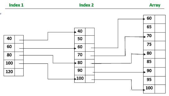
Index Searching

In this method, an index file is created containing references to groups of records. When a user requests a specific record, the search first identifies the group in the index, making the search faster.

Note: When a user makes a request for a specific record, the relevant index group is searched first, where the record is expected to be.

Characteristics

• A sorted index is maintained alongside the array.
• Each index entry points to a block of elements or another level of index.
• The index is searched first, guiding the actual search in the array.

Note: Indexed Sequential Search can create multiple levels of indexes, forming a hierarchy.

#include <iostream> 
#include <vector>   
#include <cstdlib>  
 
using namespace std;
 
void indexedSequentialSearch(int arr[], int n, int k) {
    const int GN = 3; 
    
    int elements[GN], indices[GN]; 
    int i, set = 0;
    int j = 0, ind = 0, start, end;
 
    for (i = 0; i < n; i += GN) { 
        elements[ind] = arr[i];
        indices[ind] = i;
        ind++;
        if (ind >= GN) {
            break; 
        }
    }
 
    if (k < elements[0]) {
        cout << "Not found" << endl; 
        exit(0); 
    } else {
        for (i = 1; i <= ind; i++) {
            if (k <= elements[i]) {
                start = indices[i - 1];
                end = indices[i];
                set = 1; 
                break;
            }
        }
    }
 
    if (set == 0) {
        start = indices[ind - 1]; 
        end = n; 
    }
 
    for (i = start; i < end; i++) {
        if (k == arr[i]) {
            j = 1; 
            break;
        }
    }
 
    if (j == 1) {
        cout << "Found at index " << i << endl;
    } else {
        cout << "Not found" << endl;
    }
}
 
int main() {
    int arr[] = {6, 7, 8, 9, 10, 11, 12, 13, 14, 15};
    int n = sizeof(arr) / sizeof(arr[0]);
    int k = 8;
    
    indexedSequentialSearch(arr, n, k);
 
    return 0; 
}

Output

Found at index 2

Advantages:

• Efficiency: Faster than sequential search, especially for large datasets.
• Random Access: Direct access based on keys.
• Scalability: Performance remains stable as the dataset grows.

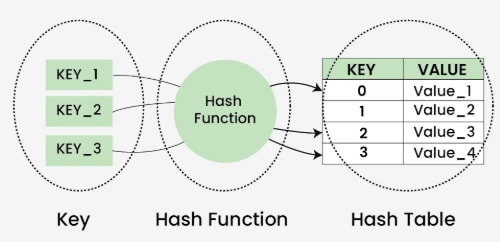
Hash Table Methods

A hash table is a data structure used to quickly insert, look up, and remove key-value pairs. It operates on the concept of hashing, where each key is translated by a hash function into a distinct index in an array. This index functions as the storage location for the corresponding value. In simple terms, it maps keys to values.

A hash table’s load factor is determined by how many elements are stored in relation to the table’s size. A high load factor can lead to longer search times and more collisions. A good hash function and proper table resizing help maintain an ideal load factor.

A function that translates keys into array indices is known as a hash function. A good hash function evenly distributes keys across the array to reduce collisions and ensure fast lookup speeds.

• Integer universe assumption: This assumes keys are integers within a certain range, enabling the use of basic hashing operations like division or multiplication hashing.
• Hashing by division: This simple technique uses the remainder of the key divided by the array size as the index. It performs well when the array size is a prime number and keys are evenly distributed.
• Hashing by multiplication: This method multiplies the key by a constant between 0 and 1, then uses the fractional part of the result. The index is obtained by multiplying this fraction by the array size. It works effectively when keys are uniformly distributed.

Methods

1. Insert (Put / Add)

   • Purpose: Adds a key-value pair to the hash table.
   • Operation: Hash the key → compute the index → insert the pair at that index (handle collisions if necessary).

2. Search (Get / Lookup)

   • Purpose: Retrieves the value associated with a given key.
   • Operation: Hash the key → compute the index → search for the key in that bucket → return the value.

3. Delete (Remove)

   • Purpose: Removes a key-value pair from the hash table.
   • Operation: Hash the key → compute the index → locate the key and remove the entry.

4. Hash Function

   • Purpose: Converts a key into an index (usually an integer).
   • A good hash function distributes keys uniformly to reduce collisions.

5. Collision Handling Techniques

   • Chaining: Stores multiple elements at the same index using a linked list or list.
   • Open Addressing: Probes to find the next available slot (e.g., linear probing, quadratic probing, double hashing).

6. Resize / Rehash

   • Purpose: Increases the hash table size when the load factor becomes too high.
   • Operation: Create a larger table and re-insert all existing key-value pairs.

7. Contains Key

   • Purpose: Checks whether a key exists in the hash table.

8. Size / Length

   • Purpose: Returns the number of key-value pairs in the table.

#include <bits/stdc++.h>
using namespace std;
 
struct Hash {
    int BUCKET; // Number of buckets
 
    // Vector of vectors to store the chains
    vector<vector<int>> table;
 
    // Constructor to initialize bucket count and table
    Hash(int b) {
        this->BUCKET = b;
        table.resize(BUCKET);
    }
 
    // Inserts a key into the hash table
    void insertItem(int key) {
        int index = hashFunction(key);
        table[index].push_back(key);
    }
 
    // Deletes a key from the hash table
    void deleteItem(int key);
 
    // Hash function to map values to keys
    int hashFunction(int x) {
        return (x % BUCKET);
    }
 
    void displayHash();
};
 
// Function to delete a key from the hash table
void Hash::deleteItem(int key) {
    int index = hashFunction(key);
 
    // Find and remove the key from table[index]
    auto it = find(table[index].begin(), table[index].end(), key);
    if (it != table[index].end()) {
        table[index].erase(it); // Erase the key if found
    }
}
 
// Function to display the hash table
void Hash::displayHash() {
    for (int i = 0; i < BUCKET; i++) {
        cout << i;
        for (int x : table[i]) {
            cout << " --> " << x;
        }
        cout << endl;
    }
}
 
// Driver program
int main() {
    // Vector that contains keys to be mapped
    vector<int> a = {15, 11, 27, 8, 12};
 
    // Insert the keys into the hash table
    Hash h(7); // 7 is the number of buckets 
    for (int key : a)
        h.insertItem(key);
 
    // Delete 12 from the hash table
    h.deleteItem(12);
 
    // Display the hash table
    h.displayHash();
 
    return 0;
}

Output

0
1 --> 15 --> 8
2
3
4 --> 11
5
6 --> 27