Bubble Sorting

Bubble Sort is the simplest sorting algorithm that works by repeatedly swapping adjacent elements if they are in the wrong order. This algorithm is not suitable for large data sets as its average and worst-case time complexities are quite high.

• We sort the array using multiple passes. After the first pass, the maximum element moves to the end (its correct position). Similarly, after the second pass, the second-largest element moves to the second-last position, and so on.
• In every pass, we process only those elements that have not already moved to their correct positions. After k passes, the largest k elements will have been moved to the last k positions.
• In a pass, we consider the remaining elements and compare all adjacent elements, swapping them if a larger element is before a smaller one. By continuing this process, the largest (among the remaining elements) ends up in its correct position. Below is the implementation of Bubble Sort. It can be optimized by stopping the algorithm if the inner loop does not cause any swap.

#include <bits/stdc++.h>
using namespace std;
 
// An optimized version of Bubble Sort 
void bubbleSort(vector<int>& arr) {
    int n = arr.size();
    bool swapped;
 
    for (int i = 0; i < n - 1; i++) {
        swapped = false;
        for (int j = 0; j < n - i - 1; j++) {
            if (arr[j] > arr[j + 1]) {
                swap(arr[j], arr[j + 1]);
                swapped = true;
            }
        }
 
        // If no two elements were swapped, break
        if (!swapped)
            break;
    }
}
 
// Function to print a vector
void printVector(const vector<int>& arr) {
    for (int num : arr)
        cout << " " << num;
}
 
int main() {
    vector<int> arr = {64, 34, 25, 12, 22, 11, 90};
    bubbleSort(arr);
    cout << "Sorted array: \n";
    printVector(arr);
    return 0;
}

Output

Sorted array: 
 11 12 22 25 34 64 90

Advantages

• Bubble Sort is easy to understand and implement.
• It does not require any additional memory space.
• It is a stable sorting algorithm, meaning elements with the same key value maintain their relative order in the sorted output.

Disadvantages

• Bubble Sort has a time complexity of O(n²), making it very slow for large data sets.
• It has almost no or very limited real-world applications and is mostly used in academics to teach sorting concepts.

Insertion Sort

Insertion sort is a simple sorting algorithm that works by iteratively inserting each element of an unsorted list into its correct position in the sorted portion of the list. It is like sorting playing cards in your hands. You split the cards into two groups: the sorted cards and the unsorted cards. Then, you pick a card from the unsorted group and put it in the right place in the sorted group.

• We start with the second element of the array, as the first element is assumed to be sorted.
• Compare the second element with the first; if it is smaller, swap them.
• Move to the third element, compare it with the first two elements, and insert it in its correct position.
• Repeat this process until the entire array is sorted.

Example: arr = {23, 1, 10, 5, 2}

• Current element: 23
• The first element in the array is assumed to be sorted.
• The sorted part up to the 0th index: [23]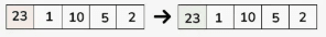
  

Step 1:

• Compare 1 with 23 (current element with the sorted part).
• Since 1 is smaller, insert 1 before 23.
• The sorted part up to the 1st index: [1, 23]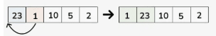
  

Step 2:

• Compare 10 with 1 and 23.
• Since 10 is greater than 1 and smaller than 23, insert 10 between 1 and 23.
• The sorted part up to the 2nd index: [1, 10, 23]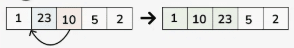
  

Step 3:

• Compare 5 with 1, 10, and 23.
• Since 5 is greater than 1 and smaller than 10, insert 5 between 1 and 10.
• The sorted part up to the 3rd index: [1, 5, 10, 23]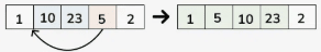
  

Step 4:

• Compare 2 with 1, 5, 10, and 23.
• Since 2 is greater than 1 and smaller than 5, insert 2 between 1 and 5.
• The sorted part up to the 4th index: [1, 2, 5, 10, 23]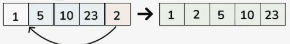
  

Step 5:

• The sorted array is: [1, 2, 5, 10, 23]

// C++ program for implementation of Insertion Sort
#include <iostream>
using namespace std;
 
/* Function to sort array using insertion sort */
void insertionSort(int arr[], int n)
{
    for (int i = 1; i < n; ++i) {
        int key = arr[i];
        int j = i - 1;
 
        /* Move elements of arr[0..i-1], that are
           greater than key, to one position ahead
           of their current position */
        while (j >= 0 && arr[j] > key) {
            arr[j + 1] = arr[j];
            j = j - 1;
        }
        arr[j + 1] = key;
    }
}
 
/* A utility function to print array of size n */
void printArray(int arr[], int n)
{
    for (int i = 0; i < n; ++i)
        cout << arr[i] << " ";
    cout << endl;
}
 
// Driver method
int main()
{
    int arr[] = { 12, 11, 13, 5, 6 };
    int n = sizeof(arr) / sizeof(arr[0]);
 
    insertionSort(arr, n);
    printArray(arr, n);
 
    return 0;
}

Output

5 6 11 12 13

Advantages

• Simple and easy to implement.
• Stable sorting algorithm.
• Efficient for small lists and nearly sorted lists.
• Space-efficient as it is an in-place algorithm.
• Adaptive: the number of inversions is directly proportional to the number of swaps. For example, no swapping occurs for a sorted array, and it takes only O(n) time.

Disadvantages

• Inefficient for large lists.
• Not as efficient as other sorting algorithms (e.g., merge sort, quick sort) in most cases.

Selection Sort

Selection Sort is a comparison-based sorting algorithm. It sorts an array by repeatedly selecting the smallest (or largest) element from the unsorted portion and swapping it with the first unsorted element. This process continues until the entire array is sorted.

1. First, we find the smallest element and swap it with the first element. This way, we place the smallest element in its correct position.
2. Then, we find the smallest among the remaining elements (i.e., the second smallest) and swap it with the second element.
3. We keep doing this until all elements are moved to their correct positions.

// C++ program to implement Selection Sort
#include <bits/stdc++.h>
using namespace std;
 
void selectionSort(vector<int> &arr) {
    int n = arr.size();
 
    for (int i = 0; i < n - 1; ++i) {
 
        // Assume the current position holds
        // the minimum element
        int min_idx = i;
 
        // Iterate through the unsorted portion
        // to find the actual minimum
        for (int j = i + 1; j < n; ++j) {
            if (arr[j] < arr[min_idx]) {
 
                // Update min_idx if a smaller
                // element is found
                min_idx = j; 
            }
        }
 
        // Move minimum element to its
        // correct position
        swap(arr[i], arr[min_idx]);
    }
}
 
void printArray(vector<int> &arr) {
    for (int &val : arr) {
        cout << val << " ";
    }
    cout << endl;
}
 
int main() {
    vector<int> arr = {64, 25, 12, 22, 11};
 
    cout << "Original array: ";
    printArray(arr); 
 
    selectionSort(arr);
 
    cout << "Sorted array: ";
    printArray(arr);
 
    return 0;
}

Output

Original vector: 64 25 12 22 11
Sorted vector: 11 12 22 25 64

Advantages

• Easy to understand and implement, making it ideal for teaching basic sorting concepts.
• Requires only constant O(1) extra memory space.
• Performs fewer swaps (or memory writes) compared to many other standard algorithms. Only cycle sort beats it in terms of memory writes. Therefore, it can be a suitable choice when memory writes are costly.

Disadvantages

• Selection Sort has a time complexity of O(n²), which makes it slower compared to algorithms like Quick Sort or Merge Sort.
• It does not maintain the relative order of equal elements, which means it is not stable.

Applications

• Perfect for teaching fundamental sorting mechanisms and algorithm design.
• Suitable for small lists where the overhead of more complex algorithms isn’t justified and memory writing is costly, as it requires fewer memory writes.
• The Heap Sort algorithm is based on Selection Sort.

Shell Sort

Shell Sort is mainly a variation of Insertion Sort. In Insertion Sort, we move elements only one position ahead. When an element has to be moved far ahead, many movements are involved. The idea of Shell Sort is to allow the exchange of far-apart items. In Shell Sort, we make the array h-sorted for a large value of h and keep reducing the value of h until it becomes 1. An array is said to be h-sorted if all sublists of every h-th element are sorted.

Algorithm:

1. Start
2. Initialize the value of the gap size, say h.
3. Divide the list into smaller sub-parts. Each must have equal intervals of h.
4. Sort these sublists using Insertion Sort.
5. Repeat step 2 until the list is sorted.
6. Print the sorted list.
7. Stop.

// C++ implementation of Shell Sort
#include <iostream>
using namespace std;
 
/* Function to sort arr using shellSort */
int shellSort(int arr[], int n) {
    // Start with a big gap, then reduce the gap
    for (int gap = n/2; gap > 0; gap /= 2) {
        // Do a gapped insertion sort for this gap size.
        for (int i = gap; i < n; i++) {
            int temp = arr[i];
            int j;
 
            // Shift earlier gap-sorted elements up until
            // the correct location for arr[i] is found
            for (j = i; j >= gap && arr[j - gap] > temp; j -= gap)
                arr[j] = arr[j - gap];
 
            // Put temp (the original arr[i]) in its correct location
            arr[j] = temp;
        }
    }
    return 0;
}
 
void printArray(int arr[], int n) {
    for (int i = 0; i < n; i++)
        cout << arr[i] << " ";
}
 
int main() {
    int arr[] = {12, 34, 54, 2, 3};
    int n = sizeof(arr)/sizeof(arr[0]);
 
    cout << "Array before sorting:\n";
    printArray(arr, n);
 
    shellSort(arr, n);
 
    cout << "\nArray after sorting:\n";
    printArray(arr, n);
 
    return 0;
}

Output

Array before sorting:
12 34 54 2 3
Array after sorting:
2 3 12 34 54

Merge Sort

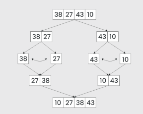
Merge Sort is a popular sorting algorithm known for its efficiency and stability. It follows the divide-and-conquer approach. It works by recursively dividing the input array into two halves, sorting the two halves individually, and finally merging them back together to obtain the sorted array.

Step-by-step explanation:

• Divide: Recursively divide the list or array into two halves until it cannot be divided further.
• Conquer: Sort each subarray individually using the Merge Sort algorithm.
• Merge: Merge the sorted subarrays back together in sorted order. This process continues until all elements are merged.

#include <bits/stdc++.h>
using namespace std;
 
// Merges two subarrays of arr[]
// First subarray is arr[left..mid]
// Second subarray is arr[mid+1..right]
void merge(vector<int>& arr, int left, int mid, int right) {
    int n1 = mid - left + 1;
    int n2 = right - mid;
 
    // Create temp vectors
    vector<int> L(n1), R(n2);
 
    // Copy data to temp vectors L[] and R[]
    for (int i = 0; i < n1; i++)
        L[i] = arr[left + i];
    for (int j = 0; j < n2; j++)
        R[j] = arr[mid + 1 + j];
 
    int i = 0, j = 0;
    int k = left;
 
    // Merge the temp vectors back into arr[left..right]
    while (i < n1 && j < n2) {
        if (L[i] <= R[j]) {
            arr[k++] = L[i++];
        } else {
            arr[k++] = R[j++];
        }
    }
 
    // Copy the remaining elements of L[], if any
    while (i < n1)
        arr[k++] = L[i++];
 
    // Copy the remaining elements of R[], if any
    while (j < n2)
        arr[k++] = R[j++];
}
 
// left is the starting index and right is the ending index
// of the subarray to be sorted
void mergeSort(vector<int>& arr, int left, int right) {
    if (left >= right)
        return;
 
    int mid = left + (right - left) / 2;
 
    mergeSort(arr, left, mid);
    mergeSort(arr, mid + 1, right);
    merge(arr, left, mid, right);
}
 
// Function to print a vector
void printVector(vector<int>& arr) {
    for (int i = 0; i < arr.size(); i++)
        cout << arr[i] << " ";
    cout << endl;
}
 
int main() {
    vector<int> arr = {12, 11, 13, 5, 6, 7};
    int n = arr.size();
 
    cout << "Given vector is\n";
    printVector(arr);
 
    mergeSort(arr, 0, n - 1);
 
    cout << "\nSorted vector is\n";
    printVector(arr);
    return 0;
}

Output

Given array is
12 11 13 5 6 7

Sorted array is
5 6 7 11 12 13

Advantages

• Stability: Merge Sort is a stable sorting algorithm, meaning it maintains the relative order of equal elements.
• Guaranteed worst-case performance: Merge Sort has a worst-case time complexity of O(n log n), which makes it efficient even on large datasets.
• Simple to implement: The divide-and-conquer approach is straightforward.
• Naturally parallel: Subarrays can be merged independently, making it suitable for parallel processing.

Disadvantages

• Space complexity: Merge Sort requires additional memory to store the merged subarrays during the sorting process.
• Not in-place: Since it uses extra space, it is not an in-place sorting algorithm, which may be a drawback in memory-constrained environments.
• Slower than Quick Sort in general: Merge Sort is usually slower than Quick Sort due to less cache efficiency, as it doesn't work entirely in-place.

Heap and Heap Sort

Heap Sort is a comparison-based sorting technique based on the Binary Heap data structure. It can be seen as an optimization over Selection Sort, where we first find the maximum (or minimum) element and swap it with the last (or first) element. We repeat the same process for the remaining elements. In Heap Sort, we use a Binary Heap so that we can quickly find and move the maximum element in O(log n) time instead of O(n), thereby achieving an overall time complexity of O(n log n).

Algorithm

First, convert the array into a Max Heap using heapify. Please note that this happens in-place. The array elements are rearranged to follow heap properties. Then, one by one, delete the root node of the Max Heap, replace it with the last node, and heapify. Repeat this process while the size of the heap is greater than 1.

• Rearrange array elements so that they form a Max Heap.

• Repeat the following steps until the heap contains only one element:

  • Swap the root element of the heap (which is the largest element in the current heap) with the last element of the heap.
  • Remove the last element of the heap (which is now in the correct position). We mainly reduce the heap size and do not remove the element from the actual array.
  • Heapify the remaining elements of the heap.

• Finally, we get the sorted array.

// C++ program for implementation of Heap Sort using vector
 
#include <bits/stdc++.h>
using namespace std;
 
// To heapify a subtree rooted with node i
// which is an index in arr[].
void heapify(vector<int>& arr, int n, int i){
 
    // Initialize largest as root
    int largest = i;
 
    // left index = 2*i + 1
    int l = 2 * i + 1;
 
    // right index = 2*i + 2
    int r = 2 * i + 2;
 
    // If left child is larger than root
    if (l < n && arr[l] > arr[largest])
        largest = l;
 
    // If right child is larger than largest so far
    if (r < n && arr[r] > arr[largest])
        largest = r;
 
    // If largest is not root
    if (largest != i) {
        swap(arr[i], arr[largest]);
 
        // Recursively heapify the affected sub-tree
        heapify(arr, n, largest);
    }
}
 
// Main function to do heap sort
void heapSort(vector<int>& arr){
    int n = arr.size();
 
    // Build heap (rearrange vector)
    for (int i = n / 2 - 1; i >= 0; i--)
        heapify(arr, n, i);
 
    // One by one extract an element from heap
    for (int i = n - 1; i > 0; i--) {
 
        // Move current root to end
        swap(arr[0], arr[i]);
 
        // Call max heapify on the reduced heap
        heapify(arr, i, 0);
    }
}
 
// A utility function to print vector of size n
void printArray(vector<int>& arr){
    for (int i = 0; i < arr.size(); ++i)
        cout << arr[i] << " ";
    cout << "\n";
}
 
// Driver's code
int main(){
    vector<int> arr = { 9, 4, 3, 8, 10, 2, 5 };
 
    // Function call
    heapSort(arr);
 
    cout << "Sorted array is \n";
    printArray(arr);
}

Output

Sorted array is 
2 3 4 5 8 9 10 

Advantages

• Efficient Time Complexity: Heap Sort has a time complexity of O(n log n) in all cases, making it efficient for sorting large datasets. The log n factor comes from the height of the binary heap, which ensures good performance even with a large number of elements.
• Memory Usage: Memory usage can be minimal (by writing an iterative heapify() instead of a recursive one). Apart from the memory required to hold the input, no additional memory is needed.
• Simplicity: It is simpler to understand than other equally efficient sorting algorithms, as it does not use advanced concepts like recursion.

Disadvantages

• Costly: Heap Sort is costly due to higher constants compared to Merge Sort, even though both have O(n log n) time complexity.
• Unstable: Heap Sort is unstable and may rearrange the relative order of equal elements.
• Inefficient: Heap Sort can be less efficient in practice due to high constant factors.

Quick Sort

Quick Sort is a sorting algorithm based on the Divide and Conquer technique. It picks an element as a pivot and partitions the given array around the chosen pivot by placing it in its correct position in the sorted array.

It works on the principle of divide and conquer, breaking down the problem into smaller sub-problems.

There are mainly three steps in the algorithm:

• Choose a Pivot: Select an element from the array as the pivot. The choice of pivot can vary (e.g., first element, last element, random element, or median).
• Partition the Array: Rearrange the array around the pivot. After partitioning, all elements smaller than the pivot will be on its left, and all elements greater than the pivot will be on its right. The pivot is then in its correct position, and we obtain its index.
• Recursively Call: Apply the same process recursively to the two partitioned sub-arrays (left and right of the pivot).
• Base Case: The recursion stops when there is only one element left in a sub-array, as a single element is already sorted.

#include <bits/stdc++.h>
using namespace std;
 
int partition(vector<int>& arr, int low, int high) {
    int pivot = arr[high];
    int i = low - 1;
 
    for (int j = low; j <= high - 1; j++) {
        if (arr[j] < pivot) {
            i++;
            swap(arr[i], arr[j]);
        }
    }
 
    swap(arr[i + 1], arr[high]);
    return i + 1;
}
 
void quickSort(vector<int>& arr, int low, int high) {
    if (low < high) {
        int pi = partition(arr, low, high);
 
        quickSort(arr, low, pi - 1);
        quickSort(arr, pi + 1, high);
    }
}
 
int main() {
    vector<int> arr = {10, 7, 8, 9, 1, 5};
    int n = arr.size();
    quickSort(arr, 0, n - 1);
 
    for (int i = 0; i < n; i++) {
        cout << arr[i] << " ";
    }
    return 0;
}

Output

Sorted Array
1 5 7 8 9 10 

Advantages

• A divide-and-conquer algorithm that simplifies complex problems.
• Efficient for large datasets.
• Low memory overhead.
• Cache-friendly due to in-place sorting.
• One of the fastest general-purpose sorting algorithms when stability is not required.
• Supports tail call optimization due to its tail-recursive nature.

Disadvantages

• Worst-case time complexity is O(n²), which occurs with poor pivot choices.
• Not ideal for small datasets.
• Not a stable sort, so equal elements may not retain their original relative positions.

Radix Sort

Radix Sort

Radix Sort is a linear-time sorting algorithm that sorts elements by processing them digit by digit. It is particularly efficient for integers or strings with fixed-size keys.

Instead of comparing elements directly, Radix Sort distributes elements into buckets based on each digit’s value. By sorting the elements repeatedly by their significant digits (from least significant to most significant), Radix Sort achieves a fully sorted array.

Radix Sort Algorithm

The core idea is to leverage the concept of place value. It assumes that sorting numbers digit by digit will eventually result in a completely sorted list. Radix Sort can be implemented in two main variations: Least Significant Digit (LSD) and Most Significant Digit (MSD) Radix Sort.

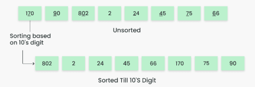
To perform Radix Sort on the array [170, 45, 75, 90, 802, 24, 2, 66], follow these steps:

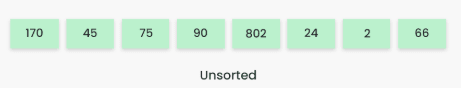
Step 1: Identify the largest element, which is 802. It has three digits, so we iterate three times—once for each digit.

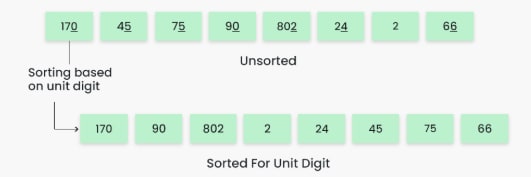
Step 2: Sort elements by unit place digits. We use a stable sorting method, such as Counting Sort. Note that the default implementation of Counting Sort is unstable, meaning elements with the same keys might not maintain their original order. To make it stable, we can iterate the input array in reverse while building the output array.

Sorting based on the unit place:

• Result: [170, 90, 802, 2, 24, 45, 75, 66]

  

Step 3: Sort elements by tens place digits.

• Result: [802, 2, 24, 45, 66, 170, 75, 90]

  

Step 4: Sort elements by hundreds place digits.

• Result: [2, 24, 45, 66, 75, 90, 170, 802]

  

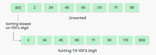
Step 5: The array is now sorted in ascending order.

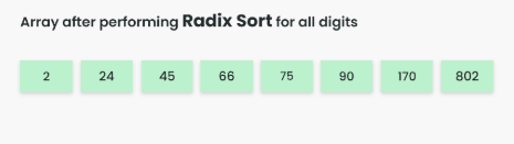
Final sorted array: [2, 24, 45, 66, 75, 90, 170, 802]

// C++ implementation of Radix Sort
 
#include <iostream>
using namespace std;
 
int getMax(int arr[], int n) {
    int mx = arr[0];
    for (int i = 1; i < n; i++)
        if (arr[i] > mx)
            mx = arr[i];
    return mx;
}
 
void countSort(int arr[], int n, int exp) {
    int output[n];
    int count[10] = {0};
 
    for (int i = 0; i < n; i++)
        count[(arr[i] / exp) % 10]++;
 
    for (int i = 1; i < 10; i++)
        count[i] += count[i - 1];
 
    for (int i = n - 1; i >= 0; i--) {
        output[count[(arr[i] / exp) % 10] - 1] = arr[i];
        count[(arr[i] / exp) % 10]--;
    }
 
    for (int i = 0; i < n; i++)
        arr[i] = output[i];
}
 
void radixsort(int arr[], int n) {
    int m = getMax(arr, n);
 
    for (int exp = 1; m / exp > 0; exp *= 10)
        countSort(arr, n, exp);
}
 
void print(int arr[], int n) {
    for (int i = 0; i < n; i++)
        cout << arr[i] << " ";
}
 
int main() {
    int arr[] = {170, 45, 75, 90, 802, 24, 2, 66};
    int n = sizeof(arr) / sizeof(arr[0]);
 
    radixsort(arr, n);
    print(arr, n);
    return 0;
}

Output

2 24 45 66 75 90 170 802 

Advantages

• Radix Sort has linear time complexity, making it faster than comparison-based algorithms like Quick Sort and Merge Sort for large datasets.
• Stable sorting: Equal elements retain their original relative order.
• Efficient for sorting large sets of integers or strings.
• Can be parallelized effectively.

Disadvantages

• Not suitable for floating-point numbers or non-digit-based data types.
• Requires extra memory for counting arrays.
• Inefficient for small datasets or datasets with few unique keys.
• Assumes that the data can be represented in a fixed number of digits.

Bucket Sort

Bucket sort is a sorting technique that involves dividing elements into various groups, or buckets. These buckets are formed by uniformly distributing the elements. Once the elements are divided into buckets, they can be sorted using any other sorting algorithm. Finally, the sorted elements are gathered together in an ordered fashion.

Algorithm

Create n empty buckets (or lists) and do the following for every array element arr[i]:

• Insert arr[i] into bucket[n * arr[i]]
• Sort individual buckets using insertion sort.
• Concatenate all sorted buckets.

Example

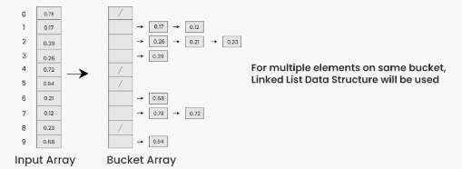
To apply bucket sort on the input array [0.78, 0.17, 0.39, 0.26, 0.72, 0.94, 0.21, 0.12, 0.23, 0.68], we follow these steps:

Step 1: Create an array of size 10, where each slot represents a bucket.

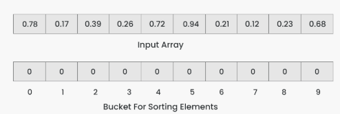
Step 2: Insert elements into the buckets from the input array based on their range. Inserting elements into the buckets:

• Take each element from the input array.
• Multiply the element by the size of the bucket array (10 in this case). For example, for element 0.23, we get 0.23 * 10 = 2.3.
• Convert the result to an integer, which gives us the bucket index. In this case, 2.3 is converted to the integer 2.
• Insert the element into the bucket corresponding to the calculated index.
• Repeat these steps for all elements in the input array.

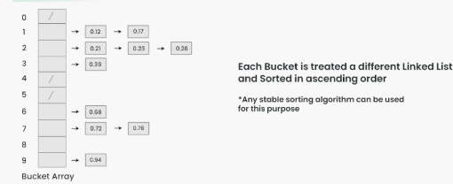
Step 3: Sort the elements within each bucket. In this example, we use quicksort (or any stable sorting algorithm) to sort the elements within each bucket. Sorting the elements within each bucket:

• Apply a stable sorting algorithm (e.g., Bubble Sort, Merge Sort) to sort the elements within each bucket.
• The elements within each bucket are now sorted.

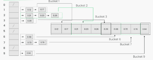
Step 4: Gather the elements from each bucket and put them back into the original array. Gathering elements from each bucket:

• Iterate through each bucket in order.
• Insert each individual element from the bucket into the original array.
• Once an element is copied, it is removed from the bucket.
• Repeat this process for all buckets until all elements have been gathered.

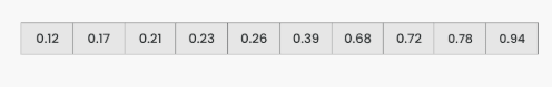
Step 5: The original array now contains the sorted elements. The final sorted array using bucket sort for the given input is [0.12, 0.17, 0.21, 0.23, 0.26, 0.39, 0.68, 0.72, 0.78, 0.94].

#include <iostream>
#include <vector>
using namespace std;
 
// Insertion sort function to sort individual buckets
void insertionSort(vector<float>& bucket) {
    for (int i = 1; i < bucket.size(); ++i) {
        float key = bucket[i];
        int j = i - 1;
        while (j >= 0 && bucket[j] > key) {
            bucket[j + 1] = bucket[j];
            j--;
        }
        bucket[j + 1] = key;
    }
}
 
// Function to sort arr[] of size n using bucket sort
void bucketSort(float arr[], int n) {
    // 1) Create n empty buckets
    vector<float> b[n];
 
    // 2) Put array elements in different buckets
    for (int i = 0; i < n; i++) {
        int bi = n * arr[i];
        b[bi].push_back(arr[i]);
    }
 
    // 3) Sort individual buckets using insertion sort
    for (int i = 0; i < n; i++) {
        insertionSort(b[i]);
    }
 
    // 4) Concatenate all buckets into arr[]
    int index = 0;
    for (int i = 0; i < n; i++) {
        for (int j = 0; j < b[i].size(); j++) {
            arr[index++] = b[i][j];
        }
    }
}
 
// Driver program to test the above function
int main() {
    float arr[] = {0.78, 0.17, 0.39, 0.26, 0.72, 0.94, 0.21, 0.12, 0.23, 0.68};
    int n = sizeof(arr) / sizeof(arr[0]);
    bucketSort(arr, n);
 
    cout << "Sorted array is\n";
    for (int i = 0; i < n; i++) {
        cout << arr[i] << " ";
    }
    return 0;
}

Output

Sorted array is 
0.12 0.17 0.21 0.23 0.26 0.39 0.68 0.72 0.78 0.94 

Address Calculation

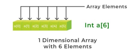
Calculating the address of any element in a 1-D array

A one-dimensional array (or single-dimensional array) is a type of linear array. Accessing its elements involves a single subscript that can represent either a row or column index.

To find the address of an element in an array, the following formula is used:

Address of A[Index] = B + W * (Index – LB)

Where:

• Index = The index of the element whose address is to be found (not the value of the element).
• B = Base address of the array.
• W = Storage size of one element in bytes.
• LB = Lower bound of the index (if not specified, assume zero).

Example: Given the base address of an array A[1300 ………… 1900] as 1020 and the size of each element is 2 bytes in memory, find the address of A[1700].

Solution:

• Base address (B) = 1020
• Lower bound (LB) = 1300
• Size of each element (W) = 2 bytes
• Index of element (not value) = 1700

Formula used:

Address of A[Index] = B + W * (Index – LB)  
Address of A[1700] = 1020 + 2 * (1700 – 1300)  
                   = 1020 + 2 * 400  
                   = 1020 + 800  
Address of A[1700] = 1820  

Calculating the address of any element in a 2-D array

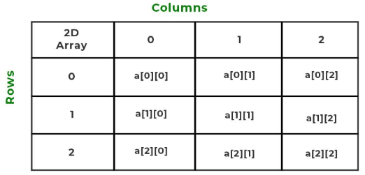
A two-dimensional array can be defined as an array of arrays. These arrays are organized as matrices represented as a collection of rows and columns in the form array[M][N], where M is the number of rows and N is the number of columns.

Example:

To find the address of any element in a 2-D array, there are two common methods:

1. Row-Major Order

Row-major ordering assigns successive memory locations across rows and then moves down to the next row. In simple terms, elements are stored in a row-wise fashion.

Formula:

Address of A[I][J] = B + W * ((I – LR) * N + (J – LC))  

I = Row index of the element  
J = Column index of the element  
B = Base address  
W = Storage size of one element (in bytes)  
LR = Lower bound of row index (assume zero if not given)  
LC = Lower bound of column index (assume zero if not given)  
N = Number of columns in the matrix  

Example: Given an array arr[1………10][1………15] with base address 100 and element size of 1 byte, find the address of arr[8][6] using row-major order.

Given:  
B = 100  
W = 1  
I = 8  
J = 6  
LR = 1  
LC = 1  
N = Upper Bound – Lower Bound + 1 = 15 – 1 + 1 = 15  

Calculation:

Address of A[8][6] = 100 + 1 * ((8 – 1) * 15 + (6 – 1))  
                   = 100 + 1 * (7 * 15 + 5)  
                   = 100 + 1 * 110  
Address = 210  

2. Column-Major Order

Column-major ordering stores elements across columns first, then down to the next column.

Formula:

Address of A[I][J] = B + W * ((J – LC) * M + (I – LR))  

M = Number of rows in the matrix  
I = Row Subset of an element whose address to be found, 
J = Column Subset of an element whose address to be found, 
B = Base address, 
W = Storage size of one element store in any array(in byte), 
LR = Lower Limit of row/start row index of matrix(If not given assume it as zero), 
LC = Lower Limit of column/start column index of matrix(If not given assume it as zero), 

Example: Given an array arr[1………10][1………15] with base address 100 and element size 1 byte, find the address of arr[8][6] using column-major order.

Given:  
B = 100  
W = 1  
I = 8  
J = 6  
LR = 1  
LC = 1  
M =  Upper Bound – Lower Bound + 1 = 10 – 1 + 1 = 10  

Calculation:

Address of A[8][6] = 100 + 1 * ((6 – 1) * 10 + (8 – 1))  
                   = 100 + 1 * (50 + 7)  
                   = 100 + 57  
Address = 157  

As seen above, for the same element, row-major and column-major orders produce different address values. This is because of the different traversal methods: row-major moves across rows first, while column-major moves down columns first.

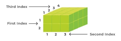
Calculating the address of any element in a 3-D array

A 3-dimensional array is a collection of 2-D arrays, represented using three subscripts:

• Block (depth)
• Row
• Column

Example:

To calculate the address in a 3-D array, we use either row-major or column-major order:

1. Row-Major Order

In row-major order, elements are stored such that columns are contiguous, then rows, then blocks.

Formula:

Address of A[i][j][k] = B + W * ((i – x) * M * N + (j – y) * N + (k – z))

Where:

• i = block index (depth)
• j = row index
• k = column index
• B = Base address
• W = Size of one element (in bytes)
• M = Number of rows per block
• N = Number of columns per row
• x = Lower bound of block index
• y = Lower bound of row index
• z = Lower bound of column index

Example: Given arr[1:9, -4:1, 5:10], base = 400, element size = 2 bytes, find address of arr[5][-1][8]

Given:
i = 5, j = -1, k = 8
x = 1, y = -4, z = 5
B = 400, W = 2
M (row count) = 1 – (–4) + 1 = 6
N (column count) = 10 – 5 + 1 = 6

Calculation:

Address = 400 + 2 * ((5 – 1) * 6 * 6 + (-1 – (–4)) * 6 + (8 – 5))
        = 400 + 2 * (144 + 18 + 3)
        = 400 + 2 * 165
        = 400 + 330
Address = 730

2. Column-Major Order

In column-major order, elements are stored such that blocks are contiguous within rows, and rows are contiguous within columns.

Formula:

Address of A[i][j][k] = B + W * ((k – z) * M * D + (j – y) * D + (i – x))

Where:

• i = block index (depth)
• j = row index
• k = column index
• B = Base address
• W = Storage size of one element (in bytes)
• M = Number of rows per block
• D = Number of blocks (depth-wise)
• x = Lower bound of block index
• y = Lower bound of row index
• z = Lower bound of column index

Example: Given arr[1:8, -5:5, -10:5], base = 400, element size = 4 bytes, find address of arr[3][3][3]

Given:
i = 3, j = 3, k = 3
x = 1, y = -5, z = -10
B = 400, W = 4
D (depth) = 8 – 1 + 1 = 8
M (rows) = 5 – (–5) + 1 = 11

Calculation:

Address = 400 + 4 * ((3 – (–10)) * 11 * 8 + (3 – (–5)) * 8 + (3 – 1))
        = 400 + 4 * (13 * 88 + 8 * 8 + 2)
        = 400 + 4 * (1144 + 64 + 2)
        = 400 + 4 * 1210
        = 400 + 4840
Address = 5240