Terminology

A Binary Tree is a hierarchical data structure in which each node has at most two children, referred to as the left child and the right child. It is commonly used in computer science for efficient storage and retrieval of data, with various operations such as insertion, deletion, and traversal.

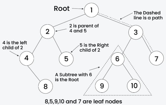
Key terminology associated with binary trees includes root, leaf, parent, child, sibling, subtree, level, height, and depth.

• Node: The fundamental unit of a tree, containing data and pointers to its children (if any).
• Root: The topmost node in the tree.
• Leaf: A node with no children.
• Parent: A node that has one or more child nodes.
• Child: A node that is a descendant of another node.
• Sibling: Nodes that share the same parent.
• Subtree: A tree that is part of a larger tree, with its root being a node in the larger tree.

Representation

Each node in a Binary Tree has three parts:

• Data

• Pointer to the left child

• Pointer to the right child

  

// Use either of the following methods to implement nodes of a binary tree
 
// 1: Using struct
struct Node {
    int data;
    Node* left, * right;
 
    Node(int key) {
        data = key;
        left = nullptr;
        right = nullptr;
    }
};
 
// 2: Using class
class Node {
public:
    int data;
    Node* left, * right;
 
    Node(int key) {
        data = key;
        left = nullptr;
        right = nullptr;
    }
};

Example

Here’s an example of creating a Binary Tree with four nodes (2, 3, 4, 5):

#include <iostream>
using namespace std;
 
struct Node{
    int data;
    Node *left, *right;
    Node(int d){
        data = d;
        left = nullptr;
        right = nullptr;
    }
};
 
int main(){
    // Initialize and allocate memory for tree nodes
    Node* firstNode = new Node(2);
    Node* secondNode = new Node(3);
    Node* thirdNode = new Node(4);
    Node* fourthNode = new Node(5);
 
    // Connect binary tree nodes
    firstNode->left = secondNode;
    firstNode->right = thirdNode;
    secondNode->left = fourthNode;
    return 0;
}

In the above code, we created four tree nodes—firstNode, secondNode, thirdNode, and fourthNode—with values 2, 3, 4, and 5, respectively.

• After creating the nodes, we connected them to form the tree structure as shown in the image above.
• Connect secondNode to the left of firstNode using firstNode->left = secondNode
• Connect thirdNode to the right of firstNode using firstNode->right = thirdNode
• Connect fourthNode to the left of secondNode using secondNode->left = fourthNode

Binary Tree Traversal

Binary trees are fundamental data structures in computer science, and understanding their traversal is crucial for various applications. Traversing a binary tree means visiting all the nodes in a specific order. There are several traversal methods, each with its own applications and benefits.

Types of Binary Tree Traversal

1. In-Order Binary Tree Traversal

In in-order traversal, the left child is visited first, followed by the node itself, and then the right child. This can be visualized as Left - Root - Right.

#include <iostream>
using namespace std;
 
class Node {
public:
    int data;
    Node* left;
    Node* right;
 
    Node(int item) {
        data = item;
        left = right = nullptr;
    }
};
 
class Eniv {
public:
    static void inOrderTraversal(Node* root) {
        if (root == nullptr) return;
 
        // Traverse the left subtree
        inOrderTraversal(root->left);
 
        // Visit the root node
        cout << root->data << " ";
 
        // Traverse the right subtree
        inOrderTraversal(root->right);
    }
};
 
int main() {
    Node* root = new Node(2);
    root->left = new Node(1);
    root->right = new Node(3);
    root->left->left = new Node(4);
    root->left->right = new Node(5);
 
    cout << "In-Order Traversal: ";
    Eniv::inOrderTraversal(root);
    cout << endl;
 
    return 0;
}

Output

In-Order Traversal: 4 1 5 2 3 

• Time Complexity: O(N)
• Auxiliary Space: O(1) if the stack space is not considered, otherwise O(h), where h is the height of the tree.

2. Pre-Order Binary Tree Traversal

In pre-order traversal, the node is visited first, followed by its left child and then its right child. This can be visualized as Root - Left - Right.

#include <iostream>
using namespace std;
 
struct Node {
    int data;
    Node* left;
    Node* right;
 
    Node(int data) {
        this->data = data;
        this->left = nullptr;
        this->right = nullptr;
    }
};
 
void preOrderTraversal(Node* root) {
    if (root == nullptr) return;
 
    // Visit the root node
    cout << root->data << " ";
 
    // Traverse the left subtree
    preOrderTraversal(root->left);
 
    // Traverse the right subtree
    preOrderTraversal(root->right);
}
 
int main() {
    // Create the following binary tree
    //       1
    //      / \
    //     2   3
    //    / \
    //   4   5
 
    Node* root = new Node(1);
    root->left = new Node(2);
    root->right = new Node(3);
    root->left->left = new Node(4);
    root->left->right = new Node(5);
 
    cout << "Pre-Order Traversal: ";
    preOrderTraversal(root);
    cout << endl;
 
    return 0;
}

Output

Pre-Order Traversal: 1 2 4 5 3 

• Time Complexity: O(N)
• Auxiliary Space: O(1) if the stack space is not considered, otherwise O(h)

3. Post-Order Binary Tree Traversal

In post-order traversal, the left child is visited first, then the right child, and finally the node itself. This can be visualized as Left - Right - Root.

#include <iostream>
using namespace std;
 
struct Node {
    int data;
    Node* left;
    Node* right;
 
    Node(int data) {
        this->data = data;
        this->left = nullptr;
        this->right = nullptr;
    }
};
 
void postOrderTraversal(Node* root) {
    if (root == nullptr) return;
 
    // Traverse the left subtree
    postOrderTraversal(root->left);
 
    // Traverse the right subtree
    postOrderTraversal(root->right);
 
    // Visit the root node
    cout << root->data << " ";
}
 
int main() {
    // Create the following binary tree
    //       1
    //      / \
    //     2   3
    //    / \
    //   4   5
 
    Node* root = new Node(1);
    root->left = new Node(2);
    root->right = new Node(3);
    root->left->left = new Node(4);
    root->left->right = new Node(5);
 
    cout << "Post-Order Traversal: ";
    postOrderTraversal(root);
    cout << endl;
 
    return 0;
}

Output

Post-Order Traversal: 4 5 2 3 1 

4. Level-Order Binary Tree Traversal

In level-order traversal, the nodes are visited level by level, starting from the root and moving to the next level. This can be visualized as Level 1 - Level 2 - Level 3 - ...

#include <iostream>
#include <queue>
using namespace std;
 
struct Node {
    int data;
    Node* left;
    Node* right;
 
    Node(int data) {
        this->data = data;
        this->left = nullptr;
        this->right = nullptr;
    }
};
 
void levelOrderTraversal(Node* root) {
    if (root == nullptr) return;
 
    queue<Node*> q;
    q.push(root);
 
    while (!q.empty()) {
        Node* current = q.front();
        q.pop();
 
        // Visit the node
        cout << current->data << " ";
 
        // Enqueue left child
        if (current->left != nullptr) q.push(current->left);
 
        // Enqueue right child
        if (current->right != nullptr) q.push(current->right);
    }
}
 
int main() {
    // Create the following binary tree
    //       1
    //      / \
    //     2   3
    //    / \
    //   4   5
 
    Node* root = new Node(1);
    root->left = new Node(2);
    root->right = new Node(3);
    root->left->left = new Node(4);
    root->left->right = new Node(5);
 
    cout << "Level-Order Traversal: ";
    levelOrderTraversal(root);
    cout << endl;
 
    return 0;
}

Output

Level-Order Traversal: 1 2 3 4 5

Binary Search Tree

A Binary Search Tree (BST) is a data structure used in computer science for organizing and storing data in a sorted manner. A BST follows all the properties of a binary tree, and for every node, its left subtree contains values less than the node, while the right subtree contains values greater than the node. This hierarchical structure allows for efficient searching, insertion, and deletion operations on the data stored in the tree.

Properties of a Binary Search Tree:

• The left subtree of a node contains only nodes with keys less than the node’s key.
• The right subtree of a node contains only nodes with keys greater than the node’s key.
• The left and right subtrees must also be binary search trees.
• There must be no duplicate nodes (although some BST variants allow duplicates with different handling strategies).

Advantages of a Binary Search Tree (BST):

• Efficient searching: O(log n) time complexity for searching in a self-balancing BST.
• Ordered structure: Elements are stored in sorted order, making it easy to find the next or previous element.
• Dynamic insertion and deletion: Elements can be added or removed efficiently.
• Balanced structure: Balanced BSTs maintain logarithmic height, ensuring efficient operations.
• Double-ended priority queue: A BST allows efficient access to both minimum and maximum elements.

Disadvantages of a Binary Search Tree (BST):

• Not self-balancing: An unbalanced BST can degrade performance.
• Worst-case time complexity: In the worst case, BST operations can take linear time.
• Memory overhead: BSTs require additional memory to store pointers to child nodes.
• Not suitable for large datasets: BSTs may become inefficient for very large datasets if not balanced.
• Limited functionality: BSTs support only basic operations like searching, insertion, and deletion.

Insertion

A new key is always inserted at a leaf while maintaining the properties of the binary search tree. We start the search for the key from the root until we reach a leaf node. Once a leaf node is found, the new node is added as its child. The steps to insert a node into a BST are as follows:

• Initialize the current node (e.g., currNode or node) with the root.

• Compare the key with the current node's value.

• Move left if the key is less than or equal to the current node’s value.

• Move right if the key is greater than the current node’s value.

• Repeat steps 2 to 4 until you reach a leaf node.

• Attach the new key as a left or right child based on the comparison with the leaf node’s value.

  

#include <iostream>
using namespace std;
 
struct Node {
    int key;
    Node* left;
    Node* right;    
    Node(int item) {
        key = item;
        left = NULL;
        right = NULL;
    }
};
 
// A utility function to insert a new node with the given key
Node* insert(Node* node, int key) {
    if (node == NULL) 
        return new Node(key);    
 
    if (node->key == key) 
        return node;
 
    if (node->key < key) 
        node->right = insert(node->right, key);
    else 
        node->left = insert(node->left, key);
 
    return node;
}
 
// A utility function to do inorder tree traversal
void inorder(Node* root) {
    if (root != NULL) {
        inorder(root->left);
        cout << root->key << " ";
        inorder(root->right);
    }
}
 
// Driver program to test the above functions
int main() {
    Node* root = new Node(50);
    root = insert(root, 30);
    root = insert(root, 20);
    root = insert(root, 40);
    root = insert(root, 70);
    root = insert(root, 60);
    root = insert(root, 80);
 
    inorder(root);
 
    return 0;
}

Output:

20 30 40 50 60 70 80 

Time Complexity:

• Worst-case time complexity of insertion is O(h), where h is the height of the BST.
• In the worst case (e.g., a skewed tree), the height becomes n, and the time complexity becomes O(n).
• Auxiliary Space: O(1)

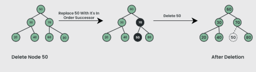
Deletion

Deletion of a node in a binary search tree can be broken down into three scenarios:

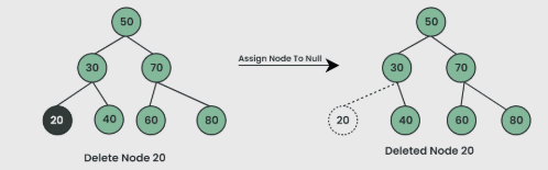
Case 1: Delete a Leaf Node in BST

Case 2: Delete a Node with One Child in BST

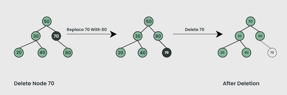
Case 3: Delete a Node with Two Children in BST

#include <bits/stdc++.h>
using namespace std;
 
struct Node {
    int key;
    Node* left;
    Node* right;
    Node(int k){
        key = k;
        left = right = nullptr;
    }
};
 
// Utility function to find the inorder successor
Node* getSuccessor(Node* curr){
    curr = curr->right;
    while (curr != nullptr && curr->left != nullptr)
        curr = curr->left;
    return curr;
}
 
// Function to delete a given key from the BST
Node* delNode(Node* root, int x){
    if (root == nullptr)
        return root;
 
    if (root->key > x)
        root->left = delNode(root->left, x);
    else if (root->key < x)
        root->right = delNode(root->right, x);
    else {
        if (root->left == nullptr) {
            Node* temp = root->right;
            delete root;
            return temp;
        }
 
        if (root->right == nullptr) {
            Node* temp = root->left;
            delete root;
            return temp;
        }
 
        Node* succ = getSuccessor(root);
        root->key = succ->key;
        root->right = delNode(root->right, succ->key);
    }
    return root;
}
 
// Utility function for inorder traversal
void inorder(Node* root){
    if (root != nullptr) {
        inorder(root->left);
        cout << root->key << " ";
        inorder(root->right);
    }
}
 
int main(){
    Node* root = new Node(10);
    root->left = new Node(5);
    root->right = new Node(15);
    root->right->left = new Node(12);
    root->right->right = new Node(18);
    int x = 15;
 
    root = delNode(root, x);
    inorder(root);
    return 0;
}

Output:

5 10 12 18

• Time Complexity: O(h), where h is the height of the BST.
• Auxiliary Space: O(h)

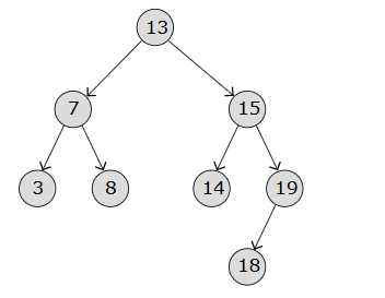
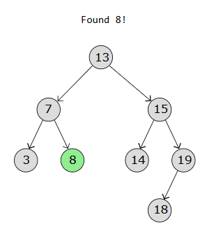
Searching

• Searching for a value in a BST is similar to performing binary search on a sorted array.
• Just like a binary search requires the array to be sorted, a BST’s structure allows for fast lookups due to its ordering property.

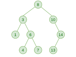
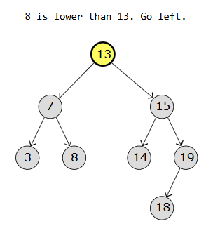
Below are diagrams showing how we search for a value (for eg 8) in a BST:

Step 1:

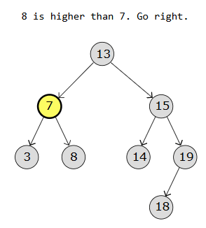
Step 2:

Step 3:

#include <iostream>
using namespace std;
 
struct Node {
    int key;
    Node* left;
    Node* right;
    Node(int item) {
        key = item;
        left = right = NULL;
    }
};
 
// Function to search a key in a BST
Node* search(Node* root, int key) {
    if (root == NULL || root->key == key)
        return root;
 
    if (root->key < key)
        return search(root->right, key);
 
    return search(root->left, key);
}
 
int main() {
    Node* root = new Node(13);
    root->left = new Node(7);
    root->right = new Node(13);
    root->left->left = new Node(3);
    root->left->right = new Node(8);
    root->right->left = new Node(14);
    root->right->right = new Node(19);
     root->right->right->left = new Node(18);
  
    (search(root, 8) != NULL) ? cout << "Found\n" : cout << "Not Found\n";
    (search(root, 80) != NULL) ? cout << "Found\n" : cout << "Not Found\n";
 
    return 0;
}

Output:

Found
Not Found

• Time Complexity: O(h), where h is the height of the BST.
• Auxiliary Space: O(h), due to the recursive call stack.

Heap Tree

A Heap is a special tree-based data structure that has the following properties:

• It is a complete binary tree.
• It follows either the max-heap or min-heap property.

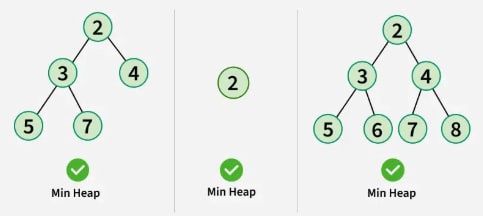
Min-Heap: The value of the root node must be the smallest among all its descendant nodes. This property must also hold true for the left and right subtrees.

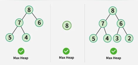
Max-Heap: The value of the root node must be the greatest among all its descendant nodes. This property must also hold true for the left and right subtrees.

Properties of a Heap:

• The minimum or maximum element is always at the root of the heap, allowing constant-time access.
• The relationship between a parent node at index i and its children is given by the formulas: left child at index 2i + 1 and right child at index 2i + 2, assuming 0-based indexing.
• Since the tree is a complete binary tree, all levels are filled except possibly the last, which is filled from left to right.
• When inserting an item, it is placed at the last available slot, then the nodes are rearranged to maintain the heap property.
• When removing an item, the root is swapped with the last node to remove either the max or min element. Then, the remaining nodes are rearranged to restore the heap property.

Implementation of Heap Data Structure:

The following code shows the implementation of a max-heap. Let’s understand the maxHeapify function in detail:

maxHeapify is the function responsible for restoring the max-heap property. It arranges node i and its subtrees to maintain the heap property:

1. Suppose we are given an array arr[] representing a complete binary tree. The left and right children of the ith node are at indices 2 * i + 1 and 2 * i + 2.
2. We set the index of the current element i as MAXIMUM.
3. If arr[2 * i + 1] > arr[i] (i.e., the left child is larger), we set it as MAXIMUM.
4. Similarly, if arr[2 * i + 2] > arr[MAXIMUM], we update MAXIMUM.
5. Swap arr[i] with arr[MAXIMUM].
6. Repeat steps 2 to 5 until the heap property is restored.

 
#include <bits/stdc++.h>
using namespace std;
 
class MaxHeap {
    int* arr;      
    int maxSize;   
    int heapSize;  
 
public:
    MaxHeap(int maxSize);
    void MaxHeapify(int);
 
    int parent(int i) { return (i - 1) / 2; }
    int lChild(int i) { return (2 * i + 1); }
    int rChild(int i) { return (2 * i + 2); }
 
    int removeMax();
    void increaseKey(int i, int newVal);
    int getMax() { return arr[0]; }
    int curSize() { return heapSize; }
 
    void deleteKey(int i);
    void insertKey(int x);
};
 
MaxHeap::MaxHeap(int totSize) {
    heapSize = 0;
    maxSize = totSize;
    arr = new int[totSize];
}
 
void MaxHeap::insertKey(int x) {
    if (heapSize == maxSize) {
        cout << "\nOverflow: Could not insertKey\n";
        return;
    }
 
    heapSize++;
    int i = heapSize - 1;
    arr[i] = x;
 
    while (i != 0 && arr[parent(i)] < arr[i]) {
        swap(arr[i], arr[parent(i)]);
        i = parent(i);
    }
}
 
void MaxHeap::increaseKey(int i, int newVal) {
    arr[i] = newVal;
    while (i != 0 && arr[parent(i)] < arr[i]) {
        swap(arr[i], arr[parent(i)]);
        i = parent(i);
    }
}
 
int MaxHeap::removeMax() {
    if (heapSize <= 0)
        return INT_MIN;
    if (heapSize == 1) {
        heapSize--;
        return arr[0];
    }
 
    int root = arr[0];
    arr[0] = arr[heapSize - 1];
    heapSize--;
 
    MaxHeapify(0);
    return root;
}
 
void MaxHeap::deleteKey(int i) {
    increaseKey(i, INT_MAX);
    removeMax();
}
 
void MaxHeap::MaxHeapify(int i) {
    int l = lChild(i);
    int r = rChild(i);
    int largest = i;
 
    if (l < heapSize && arr[l] > arr[i])
        largest = l;
    if (r < heapSize && arr[r] > arr[largest])
        largest = r;
    if (largest != i) {
        swap(arr[i], arr[largest]);
        MaxHeapify(largest);
    }
}
 
int main() {
    MaxHeap h(15);
 
    int k, i, n = 6, arr[10];
    cout << "Entered 6 keys: 3, 10, 12, 8, 2, 14\n";
    h.insertKey(3);
    h.insertKey(10);
    h.insertKey(12);
    h.insertKey(8);
    h.insertKey(2);
    h.insertKey(14);
 
    cout << "The current size of the heap is " << h.curSize() << "\n";
    cout << "The current maximum element is " << h.getMax() << "\n";
 
    h.deleteKey(2);
    cout << "The current size of the heap is " << h.curSize() << "\n";
 
    h.insertKey(15);
    h.insertKey(5);
    cout << "The current size of the heap is " << h.curSize() << "\n";
    cout << "The current maximum element is " << h.getMax() << "\n";
 
    return 0;
}

Output

Entered 6 keys: 3, 10, 12, 8, 2, 14
The current size of the heap is 6
The current maximum element is 14
The current size of the heap is 5
The current size of the heap is 7
The current maximum element is 15

Advantages of Heap Data Structure

• Time Efficient: Heaps provide an average time complexity of O(log n) for inserting and deleting elements, making them efficient for large datasets. We can convert any array to a heap in O(n) time. Most importantly, we can get the min or max in O(1) time.
• Space Efficient: A heap tree is a complete binary tree and can be stored in an array without wasting space.
• Dynamic: Heaps can be dynamically resized as elements are inserted or deleted, making them suitable for applications requiring real-time updates.
• Priority-based: Heaps allow processing elements based on priority, which is useful in real-time applications like load balancing, medical systems, and stock market analysis.
• In-place: Many heap applications require in-place element rearrangements, such as HeapSort.

Disadvantages of Heap Data Structure

• Lack of Flexibility: The heap structure is rigid, designed to maintain a specific order, and may not be suitable for applications needing more flexible data structures.
• Not Ideal for Searching: While heaps provide fast access to the top element, searching for a specific element requires O(n) time as it may involve traversing the entire structure.
• Unstable: Heaps are not stable data structures; the relative order of equal elements may not be preserved after heap operations.
• Complexity: Although insertion and deletion are efficient, some applications requiring faster algorithms may find the worst-case time complexity of O(n log n) suboptimal.

Types of Heap Trees

Different types of heap data structures include fundamental types like min heap, max heap, binary heap, and many more. In this post, we will explore their characteristics and use cases. Understanding the properties and applications of these heap data structures helps in selecting the most suitable one for a specific algorithm or application. Each type of heap has its own advantages and trade-offs, and the choice depends on the particular requirements of the problem at hand.

1. Binary Heap A binary heap is the fundamental type of heap that forms the basis for many other heap structures. It is a complete binary tree with a unique property: the value of each node is either greater than or equal to (max-heap) or less than or equal to (min-heap) the values of its children. Binary heaps are typically implemented as arrays, allowing for efficient manipulation and access.

   

   Characteristics:

   • Efficiently represented as an array.
   • Parent's value is greater than or equal to (max-heap) or less than or equal to (min-heap) children's values.

   Uses:

   • Priority queues.
   • Heap sort algorithm.

   Applications:

   • Dijkstra's shortest path algorithm.
   • Huffman coding for data compression.

2. Min Heap A min heap is a specific instance of a binary heap where the value of each node is less than or equal to the values of its children. Min heaps are particularly useful when the goal is to efficiently find and extract the minimum element from a collection.

   

   Characteristics:

   • Parent's value is less than or equal to children's values.

   Uses:

   • Efficiently finding and extracting the minimum element.

   Applications:

   • Prim's minimum spanning tree algorithm.
   • Solving the "k smallest/largest elements" problem.

3. Max Heap A max heap, on the other hand, is a binary heap where the value of each node is greater than or equal to the values of its children. Max heaps are valuable when the objective is to efficiently find and extract the maximum element from a collection.

   

   Characteristics:

   • Parent's value is greater than or equal to children's values.

   Uses:

   • Efficiently finding and extracting the maximum element.

   Applications:

   • Solving the "k smallest/largest elements" problem.

4. Binomial Heap A binomial heap extends the concept of a binary heap by introducing binomial trees. A binomial tree of order k has 2^k nodes. Binomial heaps are known for their efficient merge operations, making them valuable in certain algorithmic scenarios.

   

   Characteristics:

   • Composed of a collection of binomial trees.

   Uses:

   • Mergeable priority queues.

   Applications:

   • Efficiently merging sorted sequences.
   • Implementing graph algorithms.

5. Fibonacci Heap A Fibonacci heap is a more advanced data structure that offers better amortized time complexity for certain operations compared to traditional binary and binomial heaps. It comprises a collection of trees with a specific structure and excels in decrease-key and merge operations.

   

   Characteristics:

   • Collection of trees with specific properties.

   Uses:

   • Efficient decrease-key and merge operations.

   Applications:

   • Prim’s and Kruskal’s algorithms for minimum spanning trees.
   • Dijkstra’s shortest path algorithm.

6. D-ary Heap A D-ary heap is a generalization of the binary heap, allowing each node to have D children instead of 2. The value of D determines the arity of the heap, with the binary heap being a special case (D = 2).

   

   Characteristics:

   • Generalization of binary heap with D children per node.

   Uses:

   • Varying arity based on specific needs.

   Applications:

   • Can be tailored for specific applications requiring a particular arity.

7. Pairing Heap A pairing heap is a simpler alternative to a Fibonacci heap while still maintaining efficient time bounds for key operations. Its structure is based on a pairing mechanism, making it a suitable choice for various applications.

   

   Characteristics:

   • Trees are paired together during merge operations.

   Uses:

   • Simple design with reasonable time bounds. Applications:

   • Network optimization problems.

   • Union-find data structures.

8. Leftist Heap A leftist heap is a variant of the binary heap that introduces the “null path length” property. This property helps maintain the heap structure efficiently during merge operations.

   

   Characteristics:

   • Maintains a “null path length” property.

   Uses:

   • Efficient merge operations.

   Applications:

   • Mergeable priority queues.
   • Huffman coding.

9. Skew Heap A skew heap is another variation of the binary heap, using a specific skew-link operation to combine two heaps. It offers a different approach to heap management.

   

   Characteristics:

   • Uses skew-link operation for merging.

   Uses:

   • Simple implementation with acceptable performance.

   Applications:

   • Priority queue operations.

10. B-Heap A B-heap is a generalization of the binary heap, allowing more than two children at each node. This flexibility can be advantageous in specific scenarios.

    

    Characteristics:

    • Generalization of binary heap with more than two children per node.

    Uses:

    • Balanced trees with flexible arity.

    Applications:

    • Database indexing.
    • File systems for efficient storage management.

Operations Supported by Heap

Operations supported by min-heaps and max-heaps are the same. The only difference is that a min-heap contains the minimum element at the root of the tree, while a max-heap contains the maximum element at the root.

Heapify: This is the process of rearranging the elements to maintain the heap property. It is done either when the root is removed (we replace the root with the last node and call heapify) or when building a heap (heapify is called from the last internal node to the root). This operation takes O(log n) time.

• For a max-heap, heapify ensures the maximum element is at the root, and the property holds for all descendants.
• For a min-heap, it ensures the minimum element is at the root, and the property holds throughout.

Insertion

When a new element is inserted into the heap, it can disrupt the heap’s properties. To restore and maintain the heap structure, a heapify operation is performed. This ensures that the heap properties are preserved. Time complexity: O(log n).

Example:

Initial heap (max-heap):

           8
        /   \
      4     5
     / \
    1   2

After inserting 10:
             8
          /     \
        4       5
       / \     /
      1   2   10

After heapify (bubble up):
            10
          /    \
        4      8
       / \    /
      1   2  5

Deletion

• Deletion always removes the root element of the heap and replaces it with the last element.
• This disrupts the heap properties, so a heapify operation is needed to restore the correct structure.
• Time complexity: O(log n).

Example:

Initial heap (max-heap):

          15
        /   \
      5      7
     / \
    2   3

After deleting 15 (replace with 3 temporarily):
          3
        /   \
      5      7
     /
    2

After heapify:
          7
        /   \
      5     3
     /
    2

Heap Sort Algorithm

First, convert the array into a max-heap using heapify (in-place). Then, repeatedly remove the root node (the largest element), replace it with the last node, and call heapify. Repeat until only one element remains.

Steps:

• Rearrange array elements to form a max-heap.

• Repeat while the heap has more than one element:

  • Swap the root with the last element.
  • Remove the last element (now in the correct position).
  • Heapify the remaining elements.

• The final array is sorted.

Code:

// C++ program for Heap Sort using vector
 
#include <bits/stdc++.h>
using namespace std;
 
void heapify(vector<int>& arr, int n, int i){
    int largest = i;
    int l = 2*i + 1;
    int r = 2*i + 2;
 
    if (l < n && arr[l] > arr[largest])
        largest = l;
    if (r < n && arr[r] > arr[largest])
        largest = r;
 
    if (largest != i) {
        swap(arr[i], arr[largest]);
        heapify(arr, n, largest);
    }
}
 
void heapSort(vector<int>& arr){
    int n = arr.size();
    for (int i = n/2 - 1; i >= 0; i--)
        heapify(arr, n, i);
    for (int i = n - 1; i > 0; i--) {
        swap(arr[0], arr[i]);
        heapify(arr, i, 0);
    }
}
 
void printArray(vector<int>& arr){
    for (int x : arr) cout << x << " ";
    cout << "\n";
}
 
int main(){
    vector<int> arr = {9, 4, 3, 8, 10, 2, 5};
    heapSort(arr);
    cout << "Sorted array is\n";
    printArray(arr);
}

Output:

Sorted array is 
2 3 4 5 8 9 10

• Time Complexity: O(n log n)
• Auxiliary Space: O(log n) (due to recursion)

Introduction to AVL Trees & B-Trees

AVL Tree

An AVL tree is defined as a self-balancing Binary Search Tree (BST) where the difference between the heights of the left and right subtrees for any node is at most one.

• The absolute difference between the heights of the left and right subtrees for any node is known as the balance factor. For an AVL tree, the balance factor for all nodes must be less than or equal to 1.
• Every AVL tree is a Binary Search Tree (BST), but not every BST is an AVL tree. For example, the second diagram below is not an AVL tree.
• The main advantage of an AVL tree is that all operations (search, insert, delete, find max/min, floor, ceiling) have a time complexity of O(log n). This is because the height of an AVL tree is bounded by O(log n), whereas in a normal BST, it can grow up to O(n).
• An AVL tree maintains its balance by performing rotations during insert and delete operations to ensure both the BST property and height balance are preserved.
• Other types of self-balancing BSTs also exist, such as Red-Black Trees. Although more complex, Red-Black Trees are more commonly used in practice as they are less restrictive in terms of subtree height differences.

Example of an AVL Tree: The balance factors for different nodes are: 12: 1, 8: 1, 18: 1, 5: 1, 11: 0, 17: 0, and 4: 0. Since all differences are less than or equal to 1, the tree is an AVL tree.

Operations on an AVL Tree:

• Searching: Similar to a normal BST, with O(log n) time complexity due to the balanced structure.
• Insertion: Performs rotations along with the standard BST insertion to maintain balance.
• Deletion: Performs rotations along with standard BST deletion to maintain balance.

Advantages of AVL Trees:

• AVL trees self-balance, ensuring O(log n) time complexity for search, insert, and delete operations.
• They maintain the in-order traversal property of BSTs, enabling sorted data access.
• Due to stricter balance conditions compared to Red-Black Trees, AVL trees generally have smaller heights and provide faster search operations.
• AVL trees are relatively easier to understand and implement compared to Red-Black Trees.

Disadvantages of AVL Trees:

• More complex to implement than regular BSTs.
• Less commonly used than Red-Black Trees in practice due to stricter balancing rules, which result in more rotations during insertion and deletion.

Applications of AVL Trees:

• Widely used as the first example of a self-balancing BST in data structure courses.
• Suitable for applications with frequent lookups and rare insert/delete operations where in-order traversal, floor, ceil, min, and max operations are important.
• Red-Black Trees are often preferred in language libraries (e.g., map, set in C++, TreeMap, TreeSet in Java).
• Useful in real-time systems where consistent and predictable performance is essential.

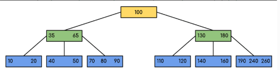
B-Tree

A B-Tree is a self-balancing m-way search tree optimized for systems that read and write large blocks of data, such as databases and file systems.

• In a B-Tree of order m, each node can have up to m children and m - 1 keys, enabling efficient management of large datasets.

• The value of m is typically chosen based on disk block size and key size.

• One of the key features of a B-Tree is its ability to store multiple keys in a single node, reducing the tree’s height and thereby minimizing expensive disk I/O operations.

• B-Trees maintain a balanced structure at all times, ensuring consistent performance for operations like search, insert, and delete.

• They allow fast and scalable data access and updates, making them ideal for use in databases and filesystems.

  

Properties of a B-Tree:

• All leaf nodes are at the same level (i.e., the tree is balanced).
• The keys in each node are stored in ascending order.
• Every internal node (except the root) has at least ⌈m/2⌉ children.
• Every node (except the root) has at least ⌈m/2⌉ - 1 keys.
• If the root is a leaf (i.e., the only node), it must have at least one key. If the root is an internal node, it must have at least two children.

Operations on a B-Tree:

• Search: Efficient due to high branching factor and balanced structure.
• Insertion: New keys are inserted into the appropriate position, and nodes may be split if they exceed the key limit.
• Deletion: Involves merging or redistributing keys to maintain B-Tree properties.

Advantages of B-Trees:

• Keeps data sorted and allows searches, insertions, deletions, and sequential access in logarithmic time.
• Reduces the number of disk reads/writes, which is crucial for performance in database systems.
• Balances itself automatically as keys are inserted or removed.

Applications of B-Trees:

• Used extensively in database indexing.
• Employed in file systems like NTFS, ext4, and HFS+.
• Used in systems requiring efficient and scalable storage management for sorted data.