Definition

It is a non-linear data structure consisting of vertices and edges. It is useful in fields such as social network analysis, recommendation systems, and computer networks. In the field of sports data science, the graph data structure can be used to analyze and understand the dynamics of team performance and player interactions on the field.

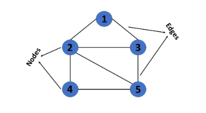
A graph is a non-linear data structure consisting of vertices and edges. The vertices are sometimes also referred to as nodes, and the edges are lines or arcs that connect any two nodes in the graph. More formally, a graph is composed of a set of vertices (V) and a set of edges (E). The graph is denoted by G(V, E).

Imagine a game of football as a web of connections, where players are the nodes and their interactions on the field are the edges. This web of connections is exactly what a graph data structure represents, and it’s the key to unlocking insights into team performance and player dynamics in sports.

Components of Graph Data Structure

• Vertices: Vertices are the fundamental units of the graph. Sometimes, vertices are also known as nodes. Every node/vertex can be labeled or unlabeled.
• Edges: Edges are used to connect two nodes of the graph. They can be ordered pairs of nodes in a directed graph. Edges can connect any two nodes in various ways. Sometimes, edges are also known as arcs. Every edge can be labeled or unlabeled.

Types of Graphs in Data Structures and Algorithms

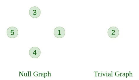
1. Null Graph A graph is known as a null graph if there are no edges in the graph.

2. Trivial Graph A graph having only a single vertex. It is also the smallest graph possible.

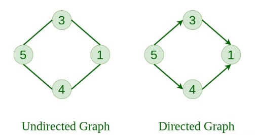
3. Undirected Graph A graph in which edges do not have any direction. That is, the nodes are unordered pairs in the definition of every edge.

4. Directed Graph A graph in which each edge has a direction. That is, the nodes are ordered pairs in the definition of every edge.

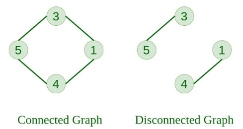
5. Connected Graph A graph in which any node can be reached from any other node is known as a connected graph.

6. Disconnected Graph A graph in which at least one node is not reachable from some other node is known as a disconnected graph.

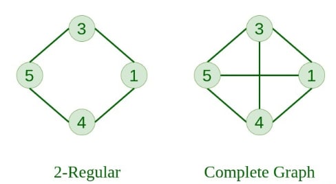
7. Regular Graph A graph in which the degree of every vertex is equal to k is called a k-regular graph.

8. Complete Graph A graph in which each node has an edge to every other node.

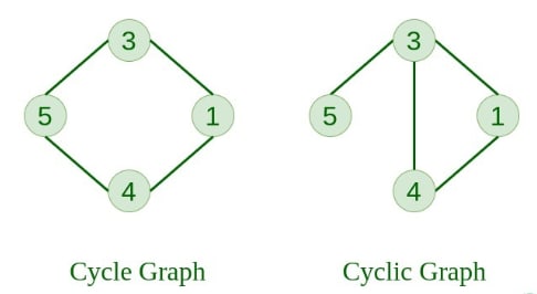
9. Cycle Graph A graph that forms a cycle. The minimum degree of each vertex is 2.

10. Cyclic Graph A graph containing at least one cycle is known as a cyclic graph.

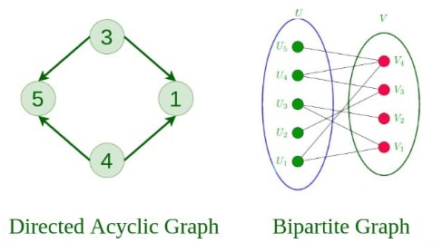
11. Directed Acyclic Graph (DAG) A directed graph that does not contain any cycles.

12. Bipartite Graph A graph in which vertices can be divided into two sets such that no two vertices within the same set are connected.

13. Weighted Graph

• A graph in which the edges have associated weights is known as a weighted graph.
• Weighted graphs can be further classified as directed weighted graphs and undirected weighted graphs.

Advantages of Graph Data Structure:

• Graphs can represent a wide range of relationships, unlike other data structures (e.g., trees cannot have cycles and must be hierarchical).
• They can be used to model and solve a wide range of problems, including pathfinding, data clustering, network analysis, and machine learning.
• Any real-world problem involving a set of items and their relationships can be easily modeled using a graph. Standard graph algorithms like BFS, DFS, Spanning Tree, Shortest Path, Topological Sorting, and Strongly Connected Components are widely applicable.
• Graphs can represent complex data structures in a simple and intuitive way, making them easier to understand and analyze.

Disadvantages of Graph Data Structure:

• Graphs can be complex and difficult to understand, especially for those unfamiliar with graph theory or related algorithms.
• Creating and manipulating graphs can be computationally expensive, particularly for very large or complex graphs.
• Graph algorithms can be challenging to design and implement correctly and are prone to bugs and errors.
• Visualizing and analyzing very large or complex graphs can be difficult, making it hard to extract meaningful insights.

Representation of Graph

There are multiple ways to store a graph. The following are the most common representations:

• Adjacency Matrix
• Adjacency List

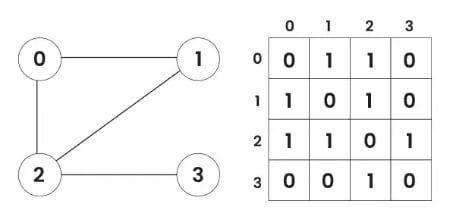
Adjacency Matrix

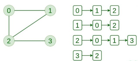
In this method, the graph is stored as a 2D matrix where rows and columns represent vertices. Each entry in the matrix represents the weight of the edge between the corresponding vertices.

Below is the implementation of a Graph represented using an Adjacency Matrix:

 
#include <bits/stdc++.h>
using namespace std;
 
void addEdge(vector<vector<int>> &mat, int i, int j) {
    mat[i][j] = 1;
    mat[j][i] = 1; 
}
 
void displayMatrix(vector<vector<int>> &mat) {
    int V = mat.size();
    for (int i = 0; i < V; i++) {
        for (int j = 0; j < V; j++)
            cout << mat[i][j] << " ";
        cout << endl;
    }
}
 
int main() {
    int V = 4;
    vector<vector<int>> mat(V, vector<int>(V, 0));
 
    addEdge(mat, 0, 1);
    addEdge(mat, 0, 2);
    addEdge(mat, 1, 2);
    addEdge(mat, 2, 3);
 
    cout << "Adjacency Matrix Representation" << endl;
    displayMatrix(mat);
 
    return 0;
}

Output:

Adjacency Matrix Representation
0 1 1 0 
1 0 1 0 
1 1 0 1 
0 0 1 0 

Adjacency List

This graph is represented as a collection of linked lists. There is an array of pointers that point to the edges connected to each vertex.

Below is the implementation of a Graph represented using an Adjacency List:

#include <iostream>
#include <vector>
using namespace std;
 
void addEdge(vector<vector<int>>& adj, int i, int j) {
    adj[i].push_back(j);
    adj[j].push_back(i); 
}
 
void displayAdjList(const vector<vector<int>>& adj) {
    for (int i = 0; i < adj.size(); i++) {
        cout << i << ": ";
        for (int j : adj[i]) {
            cout << j << " ";
        }
        cout << endl;
    }
}
 
int main() {
    int V = 4;
    vector<vector<int>> adj(V); 
 
    addEdge(adj, 0, 1);
    addEdge(adj, 0, 2);
    addEdge(adj, 1, 2);
    addEdge(adj, 2, 3);
 
    cout << "Adjacency List Representation:" << endl;
    displayAdjList(adj);
 
    return 0;
}

Output:

Adjacency List Representation:
0: 1 2 
1: 0 2 
2: 0 1 3 
3: 2 

Traversing a Graph

To traverse a graph means to start at one vertex and follow the edges to visit other vertices until all vertices (or as many as possible) have been visited.

The two most common graph traversal methods are:

• Depth First Search (DFS)
• Breadth First Search (BFS)

DFS is usually implemented using a stack or via recursion (which utilizes the call stack), while BFS is usually implemented using a queue.

DFS (Depth First Search Traversal)

Depth First Search is called "deep" because it explores a vertex, then its adjacent vertex, and continues down that path before backtracking. For example:

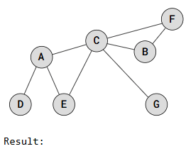
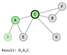
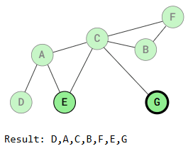
The DFS traversal starts at vertex D, marks it as visited, and recursively visits all adjacent, unvisited vertices. When vertex A is visited, traversal continues to vertex C or vertex E, depending on the implementation.

#include <iostream>
#include <vector>
#include <string>
using namespace std;
 
class Graph {
private:
    vector<vector<int>> adj_matrix;
    vector<string> vertex_data;
    int size;
 
    void dfs_util(int v, vector<bool>& visited) {
        visited[v] = true;
        cout << vertex_data[v] << " ";
 
        for (int i = 0; i < size; ++i) {
            if (adj_matrix[v][i] == 1 && !visited[i]) {
                dfs_util(i, visited);
            }
        }
    }
 
public:
    Graph(int s) {
        size = s;
        adj_matrix = vector<vector<int>>(size, vector<int>(size, 0));
        vertex_data = vector<string>(size, "");
    }
 
    void add_edge(int u, int v) {
        if (u >= 0 && u < size && v >= 0 && v < size) {
            adj_matrix[u][v] = 1;
            adj_matrix[v][u] = 1;
        }
    }
 
    void add_vertex_data(int vertex, const string& data) {
        if (vertex >= 0 && vertex < size) {
            vertex_data[vertex] = data;
        }
    }
 
    void print_graph() {
        cout << "Adjacency Matrix:\n";
        for (const auto& row : adj_matrix) {
            for (int val : row) {
                cout << val << " ";
            }
            cout << endl;
        }
 
        cout << "\nVertex Data:\n";
        for (int i = 0; i < size; ++i) {
            cout << "Vertex " << i << ": " << vertex_data[i] << endl;
        }
    }
 
    void dfs(const string& start_vertex_data) {
        vector<bool> visited(size, false);
        int start_vertex = -1;
 
        for (int i = 0; i < size; ++i) {
            if (vertex_data[i] == start_vertex_data) {
                start_vertex = i;
                break;
            }
        }
 
        if (start_vertex != -1) {
            dfs_util(start_vertex, visited);
        } else {
            cout << "Start vertex not found.\n";
        }
    }
};
 
int main() {
    Graph g(7);
 
    g.add_vertex_data(0, "A");
    g.add_vertex_data(1, "B");
    g.add_vertex_data(2, "C");
    g.add_vertex_data(3, "D");
    g.add_vertex_data(4, "E");
    g.add_vertex_data(5, "F");
    g.add_vertex_data(6, "G");
 
    g.add_edge(3, 0);  // D - A
    g.add_edge(0, 2);  // A - C
    g.add_edge(0, 3);  // A - D
    g.add_edge(0, 4);  // A - E
    g.add_edge(4, 2);  // E - C
    g.add_edge(2, 5);  // C - F
    g.add_edge(2, 1);  // C - B
    g.add_edge(2, 6);  // C - G
    g.add_edge(1, 5);  // B - F
 
    g.print_graph();
 
    cout << "\nDepth First Search starting from vertex D:\n";
    g.dfs("D");
 
    return 0;
}

Output:

Adjacency Matrix:
0 0 1 1 1 0 0 
0 0 1 0 0 1 0 
1 1 0 0 1 1 1 
1 0 0 0 0 0 0 
1 0 1 0 0 0 0 
0 1 1 0 0 0 0 
0 0 1 0 0 0 0 

Vertex Data:
Vertex 0: A
Vertex 1: B
Vertex 2: C
Vertex 3: D
Vertex 4: E
Vertex 5: F
Vertex 6: G

Depth First Search starting from vertex D:
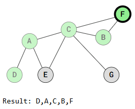
D A C B F E G 

Explanation:

• Class Design:

  • adj_matrix: 2D vector for representing graph edges.
  • vertex_data: stores a label (like 'A', 'B', etc.) for each vertex.
  • dfs_util: helper function for recursive DFS traversal.

• Functionality Mapping:

  • add_edge(u, v): Adds an undirected edge by updating both adj_matrix[u][v] and adj_matrix[v][u].
  • add_vertex_data(i, label): Assigns a string label to a vertex.
  • dfs(start_label): Begins DFS from the vertex whose label matches start_label.

• DFS Mechanism:

  • A visited array ensures we don’t visit the same vertex multiple times.
  • DFS is implemented recursively via dfs_util.

BFS (Breadth-First Search Traversal)

Breadth-First Search visits all adjacent vertices of a vertex before visiting the neighbors of those adjacent vertices. This means that vertices at the same distance from the starting vertex are visited before vertices that are farther away.

For Example:

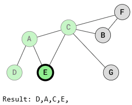
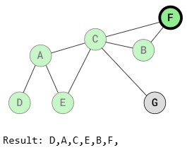
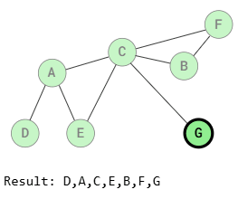
As shown in the images above, BFS traversal visits vertices that are the same distance from the starting vertex before visiting those farther away. For example, after visiting vertex A, vertices E and C are visited before B, F, and G because those vertices are farther away.

Breadth-First Search works by placing all adjacent vertices into a queue (if they haven’t already been visited) and then using the queue to visit the next vertex.

Code example for Breadth-First Search:

#include <stdio.h>
#include <stdbool.h>
 
#define SIZE 7
 
typedef struct {
    int adjMatrix[SIZE][SIZE];
    char vertexData[SIZE];
} Graph;
 
void initGraph(Graph *g) {
    for (int i = 0; i < SIZE; i++) {
        for (int j = 0; j < SIZE; j++) {
            g->adjMatrix[i][j] = 0;
        }
        g->vertexData[i] = '\0';
    }
}
 
void addEdge(Graph *g, int u, int v) {
    if (u >= 0 && u < SIZE && v >= 0 && v < SIZE) {
        g->adjMatrix[u][v] = 1;
        g->adjMatrix[v][u] = 1;
    }
}
 
void addVertexData(Graph *g, int vertex, char data) {
    if (vertex >= 0 && vertex < SIZE) {
        g->vertexData[vertex] = data;
    }
}
 
void printGraph(Graph *g) {
    printf("Adjacency Matrix:\n");
    for (int i = 0; i < SIZE; i++) {
        for (int j = 0; j < SIZE; j++) {
            printf("%d ", g->adjMatrix[i][j]);
        }
        printf("\n");
    }
 
    printf("\nVertex Data:\n");
    for (int i = 0; i < SIZE; i++) {
        printf("Vertex %d: %c\n", i, g->vertexData[i]);
    }
}
 
void bfs(Graph *g, char startVertexData) {
    bool visited[SIZE] = {false};
    int queue[SIZE], queueStart = 0, queueEnd = 0;
    int startVertex = -1;
 
    for (int i = 0; i < SIZE; i++) {
        if (g->vertexData[i] == startVertexData) {
            startVertex = i;
            break;
        }
    }
 
    if (startVertex != -1) {
        queue[queueEnd++] = startVertex;
        visited[startVertex] = true;
 
        while (queueStart < queueEnd) {
            int currentVertex = queue[queueStart++];
            printf("%c ", g->vertexData[currentVertex]);
 
            for (int i = 0; i < SIZE; i++) {
                if (g->adjMatrix[currentVertex][i] == 1 && !visited[i]) {
                    queue[queueEnd++] = i;
                    visited[i] = true;
                }
            }
        }
    }
}
 
int main() {
    Graph g;
    initGraph(&g);
 
    addVertexData(&g, 0, 'A');
    addVertexData(&g, 1, 'B');
    addVertexData(&g, 2, 'C');
    addVertexData(&g, 3, 'D');
    addVertexData(&g, 4, 'E');
    addVertexData(&g, 5, 'F');
    addVertexData(&g, 6, 'G');
 
    addEdge(&g, 3, 0); // D - A
    addEdge(&g, 0, 2); // A - C
    addEdge(&g, 0, 3); // A - D
    addEdge(&g, 0, 4); // A - E
    addEdge(&g, 4, 2); // E - C
    addEdge(&g, 2, 5); // C - F
    addEdge(&g, 2, 1); // C - B
    addEdge(&g, 2, 6); // C - G
    addEdge(&g, 1, 5); // B - F
 
    printGraph(&g);
 
    printf("\nBreadth-First Search starting from vertex D:\n");
    bfs(&g, 'D');
 
    return 0;
}

Output

Adjacency Matrix:
0 0 1 1 1 0 0
0 0 1 0 0 1 0
1 1 0 0 1 1 1
1 0 0 0 0 0 0
1 0 1 0 0 0 0
0 1 1 0 0 0 0
0 0 1 0 0 0 0

Vertex Data:
Vertex 0: A
Vertex 1: B
Vertex 2: C
Vertex 3: D
Vertex 4: E
Vertex 5: F
Vertex 6: G

Breadth-First Search starting from vertex D:
D A C E B F G

The bfs() method starts by creating a queue with the start vertex, initializing a visited array, and marking the start vertex as visited.

It then repeatedly dequeues a vertex, prints it, enqueues its unvisited adjacent vertices, and continues this process until all reachable vertices have been visited.

Dijkstra's Algorithm for Shortest Distance

Dijkstra's algorithm is a popular method for solving single-source shortest path problems in graphs with non-negative edge weights. It is used to find the shortest distance between two vertices in a graph. The algorithm was conceived by Dutch computer scientist Edsger W. Dijkstra in 1956.

The algorithm maintains two sets: one for visited vertices and another for unvisited vertices. It starts at the source vertex and iteratively selects the unvisited vertex with the smallest tentative distance from the source. Then it visits the neighbors of this vertex and updates their tentative distances if a shorter path is found. This process continues until the destination vertex is reached or all reachable vertices have been visited.

Algorithm

1. Mark the source node with a current distance of 0 and all others with infinity.
2. Set the unvisited node with the smallest current distance as the current node.
3. For each neighbor N of the current node, add the current distance of the node to the weight of the edge connecting them. If this is smaller than the current distance of N, update it.
4. Mark the current node as visited.
5. Repeat step 2 if there are still unvisited nodes.

Example: Given a weighted undirected graph represented as an edge list and a source vertex src, find the shortest path distances from the source vertex to all other vertices in the graph. The graph contains V vertices, numbered from 0 to V - 1.

Note: The given graph does not contain any negative edges.

Input: src = 0, V = 5, edges[][] = [[0, 1, 4], [0, 2, 8], [1, 4, 6], [2, 3, 2], [3, 4, 10]]

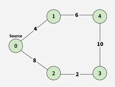
Output:

0 4 8 10 10

Explanation:

Shortest Paths:  
0 to 1 = 4 → 0 → 1  
0 to 2 = 8 → 0 → 2  
0 to 3 = 10 → 0 → 2 → 3  
0 to 4 = 10 → 0 → 1 → 4  

#include <iostream>
#include <vector>
#include <queue>
#include <climits>
using namespace std;
 
// Function to construct adjacency list
vector<vector<vector<int>>> constructAdj(vector<vector<int>> &edges, int V) {
    vector<vector<vector<int>>> adj(V); 
    for (const auto &edge : edges) {
        int u = edge[0];
        int v = edge[1];
        int wt = edge[2];
        adj[u].push_back({v, wt});
        adj[v].push_back({u, wt}); 
    }
    return adj;
}
 
// Returns shortest distances from src to all other vertices
vector<int> dijkstra(int V, vector<vector<int>> &edges, int src){
    vector<vector<vector<int>>> adj = constructAdj(edges, V);
    priority_queue<vector<int>, vector<vector<int>>, greater<vector<int>>> pq;
    vector<int> dist(V, INT_MAX);
    pq.push({0, src});
    dist[src] = 0;
 
    while (!pq.empty()){
        int u = pq.top()[1];
        pq.pop();
 
        for (auto x : adj[u]){
            int v = x[0];
            int weight = x[1];
 
            if (dist[v] > dist[u] + weight) {
                dist[v] = dist[u] + weight;
                pq.push({dist[v], v});
            }
        }
    }
 
    return dist;
}
 
int main(){
    int V = 5;
    int src = 0;
    vector<vector<int>> edges = {{0, 1, 4}, {0, 2, 8}, {1, 4, 6}, {2, 3, 2}, {3, 4, 10}};
    vector<int> result = dijkstra(V, edges, src);
 
    for (int dist : result)
        cout << dist << " ";
    return 0;
}

Output:

0 4 8 10 10

Time Complexity: O(E * log V), where E is the number of edges and V is the number of vertices. Auxiliary Space: O(V), where V is the number of vertices. (The adjacency list is excluded from auxiliary space as it is part of the input representation.)

Minimum Spanning Tree

A spanning tree is a tree-like subgraph of a connected, undirected graph that includes all the vertices of the graph. In simple terms, it is a subset of the graph’s edges that forms an acyclic structure (tree), where every node in the graph is connected.

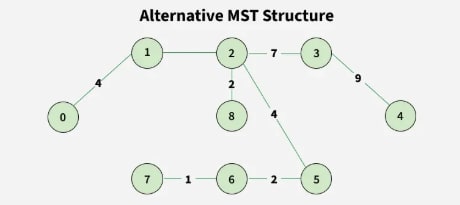
A minimum spanning tree (MST) possesses all the properties of a spanning tree, with the added requirement that the total edge weight must be the smallest among all possible spanning trees. Like spanning trees, a graph can have multiple valid MSTs.

Properties:

• The number of vertices (V) in the graph and the spanning tree is the same.
• The number of edges in the spanning tree is always one less than the number of vertices (E = V - 1).
• The spanning tree must be connected; there should be only one connected component.
• The spanning tree must be acyclic.
• The total cost (or weight) of a spanning tree is the sum of the weights of its edges.
• There can be multiple spanning trees for a graph.

Algorithms to Find Minimum Spanning Tree

Several algorithms can be used to find the MST of a graph. Some popular ones include:

Kruskal’s Minimum Spanning Tree Algorithm

A minimum spanning tree (MST) or minimum weight spanning tree for a weighted, connected, and undirected graph is a spanning tree (a tree with no cycles that connects all vertices) with the minimum possible total edge weight. The weight of a spanning tree is the sum of all the edge weights in the tree.

In Kruskal's algorithm, all edges of the given graph are first sorted in increasing order of their weights. Then, edges are added one by one to the MST if the addition of the edge does not form a cycle. It begins by selecting the edge with the smallest weight and continues up to the edge with the largest weight. Thus, it makes a locally optimal choice at each step in order to find the globally optimal solution. Hence, it is a Greedy Algorithm.

This is one of the most popular algorithms for finding the minimum spanning tree of a connected, undirected graph. The algorithm follows the Greedy approach. The workflow of the algorithm is as follows:

• First, sort all the edges of the graph by their weights.
• Then, iterate through the sorted edges.
• At each iteration, add the next lowest-weight edge, provided it does not form a cycle with the edges selected so far.

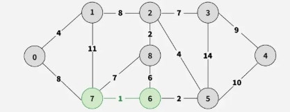
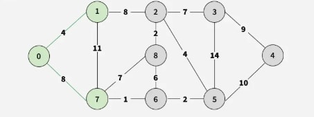
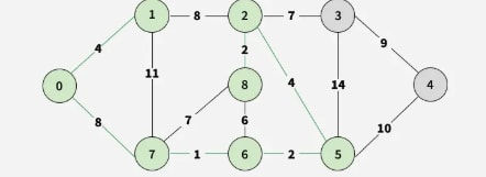
Example The graph contains 9 vertices and 14 edges. So, the minimum spanning tree formed will have (9 - 1) = 8 edges.

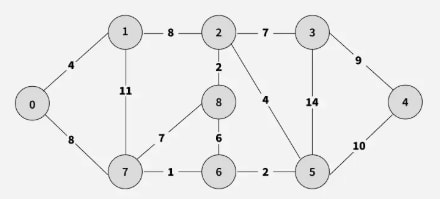
Step 1: Pick all sorted edges one by one. Pick edge 7–6. No cycle is formed, include it.

Step 2: Pick edge 8–2. No cycle is formed, include it.

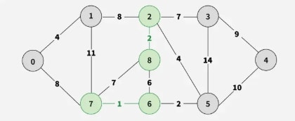
Step 3: Pick edge 6–5. No cycle is formed, include it.

Step 4: Pick edge 0–1. No cycle is formed, include it.

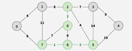
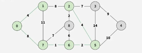
Step 5: Pick edge 2–5. No cycle is formed, include it.

Step 6: Pick edge 8–6. Since including this edge results in a cycle, discard it. Pick edge 2–3. No cycle is formed, include it.

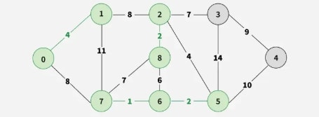
Step 7: Pick edge 7–8. Since including this edge results in a cycle, discard it. Pick edge 0–7. No cycle is formed, include it.

Step 8: Pick edge 1–2. Since including this edge results in a cycle, discard it. Pick edge 3–4. No cycle is formed, include it.

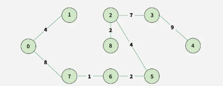
Step 9: Final obtained graph: Minimum Spanning Tree.

#include <bits/stdc++.h>
using namespace std;
 
// Disjoint set data structure
class DSU {
    vector<int> parent, rank;
 
public:
    DSU(int n) {
        parent.resize(n);
        rank.resize(n);
        for (int i = 0; i < n; i++) {
            parent[i] = i;
            rank[i] = 1;
        }
    }
 
    int find(int i) {
        return (parent[i] == i) ? i : (parent[i] = find(parent[i]));
    }
 
    void unite(int x, int y) {
        int s1 = find(x), s2 = find(y);
        if (s1 != s2) {
            if (rank[s1] < rank[s2]) parent[s1] = s2;
            else if (rank[s1] > rank[s2]) parent[s2] = s1;
            else parent[s2] = s1, rank[s1]++;
        }
    }
};
 
bool comparator(vector<int> &a, vector<int> &b) {
    return a[2] < b[2];
}
 
int kruskalsMST(int V, vector<vector<int>> &edges) {
    // Sort all edges
    sort(edges.begin(), edges.end(), comparator);
 
    // Traverse edges in sorted order
    DSU dsu(V);
    int cost = 0, count = 0;
 
    for (auto &e : edges) {
        int x = e[0], y = e[1], w = e[2];
 
        // Make sure that there is no cycle
        if (dsu.find(x) != dsu.find(y)) {
            dsu.unite(x, y);
            cost += w;
            if (++count == V - 1) break;
        }
    }
    return cost;
}
 
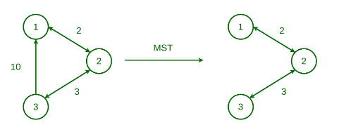
int main() {
    // Each edge contains source, destination, and weight
    vector<vector<int>> edges = {
        {0, 1, 10}, {1, 3, 15}, {2, 3, 4}, {2, 0, 6}, {0, 3, 5}
    };
 
    cout << "Minimum Cost Spanning Tree: " << kruskalsMST(4, edges) << endl;
 
    return 0;
}

Output

Minimum Cost Spanning Tree: 19

This algorithm can be implemented efficiently using a DSU (Disjoint Set Union) data structure to keep track of the connected components of the graph. It is used in a variety of practical applications such as network design, clustering, and data analysis.

Prim’s Minimum Spanning Tree Algorithm

Prim’s algorithm is a greedy algorithm like Kruskal’s algorithm. It always starts with a single node and expands through adjacent nodes to explore all the connected edges along the way.

• The algorithm starts with an empty spanning tree.
• The idea is to maintain two sets of vertices: one containing the vertices already included in the MST, and the other containing the vertices not yet included.
• At every step, it considers all the edges that connect the two sets and picks the minimum weight edge from these. After picking the edge, it adds the other endpoint of the edge to the MST set.

In graph theory, a group of edges that connects two sets of vertices in a graph is called a cut. The vertices that, when removed, increase the number of connected components are called articulation points (or cut vertices), but this is different from the edges used in Prim’s algorithm. So, at every step of Prim’s algorithm, a cut is formed, the minimum weight edge crossing the cut is selected, and the corresponding vertex is included in the MST set.

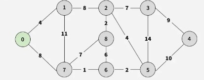
Step 1: Choose an arbitrary vertex as the starting vertex of the MST. We pick 0 in the diagram below.

Step 2: Follow steps 3 to 5 until all vertices are included in the MST (known as fringe vertices).

Step 3: Find edges connecting any tree vertex with the fringe vertices.

Step 4: Find the minimum among these edges.

Step 5: Add the chosen edge to the MST. Since we only consider edges that connect tree vertices with fringe vertices, no cycles are formed.

Step 6: Return the MST and exit.

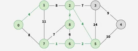
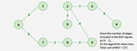
Example

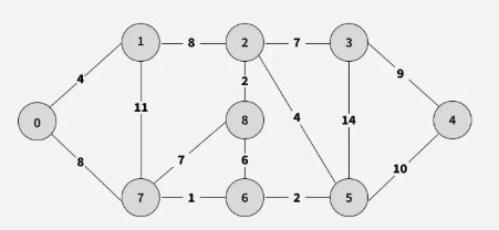
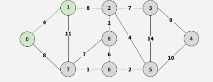
Step 1: Start with edges 0-1 and 0-7; pick the minimum 0-1 and add vertex 1.

Step 2: Choose between 0-7 and 1-2; pick 0-7 (or 1-2), adding vertex 7.

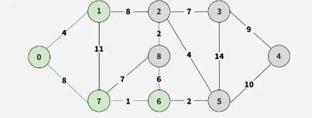
Step 3: Select 7-6 as it has the least weight (1), adding vertex 6.

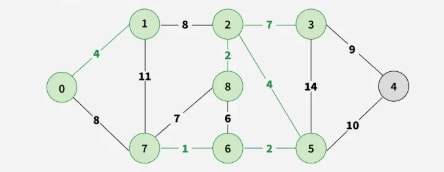
Step 4: Among 7-8, 6-8, and 6-5 (weight 2), add vertex 5.

Step 5: Select 5-2 (weight 4), adding vertex 2.

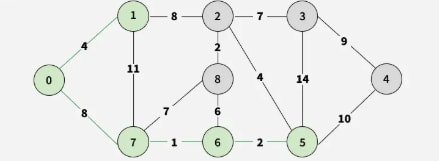
Step 6: Choose 2-8 (weight 2), adding vertex 8.

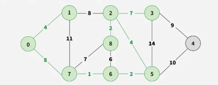
Step 7: Pick 2-3 as the smallest edge, adding vertex 3.

Step 8: Finally, select 3-4, adding vertex 4.

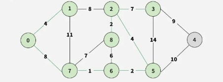
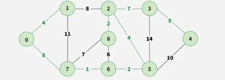
Step 9: All vertices are included, so the MST is complete.

Step 10:

// A C++ program for Prim's Minimum
// Spanning Tree (MST) algorithm. The program is
// for adjacency matrix representation of the graph
#include <bits/stdc++.h>
using namespace std;
 
// A utility function to find the vertex with
// minimum key value, from the set of vertices
// not yet included in MST
int minKey(vector<int> &key, vector<bool> &mstSet) {
    int min = INT_MAX, min_index;
 
    for (int v = 0; v < mstSet.size(); v++)
        if (!mstSet[v] && key[v] < min)
            min = key[v], min_index = v;
 
    return min_index;
}
 
// A utility function to print the
// constructed MST stored in parent[]
void printMST(vector<int> &parent, vector<vector<int>> &graph) {
    cout << "Edge \tWeight\n";
    for (int i = 1; i < graph.size(); i++)
        cout << parent[i] << " - " << i << " \t"
             << graph[parent[i]][i] << " \n";
}
 
// Function to construct and print MST for
// a graph represented using adjacency
// matrix representation
void primMST(vector<vector<int>> &graph) {
    int V = graph.size();
    vector<int> parent(V);     // Array to store constructed MST
    vector<int> key(V);        // Key values used to pick minimum weight edge in cut
    vector<bool> mstSet(V);    // To represent set of vertices included in MST
 
    for (int i = 0; i < V; i++)
        key[i] = INT_MAX, mstSet[i] = false;
 
    key[0] = 0;       // Include first vertex in MST
    parent[0] = -1;   // First node is always root of MST
 
    for (int count = 0; count < V - 1; count++) {
        int u = minKey(key, mstSet);
        mstSet[u] = true;
 
        for (int v = 0; v < V; v++)
            if (graph[u][v] && !mstSet[v] && graph[u][v] < key[v])
                parent[v] = u, key[v] = graph[u][v];
    }
 
    printMST(parent, graph);
}
 
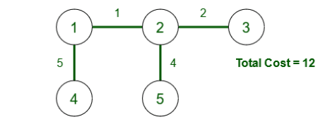
int main() {
    vector<vector<int>> graph = {
        { 0, 2, 0, 6, 0 },
        { 2, 0, 3, 8, 5 },
        { 0, 3, 0, 0, 7 },
        { 6, 8, 0, 0, 9 },
        { 0, 5, 7, 9, 0 }
    };
 
    primMST(graph);
 
    return 0;
}

Output

Edge    Weight
0 - 1   2 
1 - 2   3 
0 - 3   6 
1 - 4   5 

Advantages and Disadvantages of Prim's Algorithm

Advantages:

• Prim's algorithm is guaranteed to find the MST in a connected, weighted graph.
• It has a time complexity of O((E + V) * log(V)) using a binary heap or Fibonacci heap, where E is the number of edges and V is the number of vertices.
• It is relatively simple to understand and implement compared to some other MST algorithms.

Disadvantages:

• Like Kruskal’s algorithm, Prim’s algorithm can be slow on dense graphs with many edges, as it requires iterating over many edges.
• It relies on a priority queue, which may use additional memory and slow down on very large graphs.
• The choice of starting node can affect the structure of the MST, which may not be ideal in all applications.

Boruvka’s Minimum Spanning Tree Algorithm

This is also a graph traversal algorithm used to find the minimum spanning tree of a connected, undirected graph. It is one of the oldest MST algorithms. It works by iteratively building the MST, starting with each vertex in the graph as its own tree. In each iteration, the algorithm finds the cheapest edge that connects a tree to another tree and adds that edge to the MST. It is somewhat similar to Prim’s algorithm in its goal.

The algorithm follows this workflow:

• Initialize a forest of trees, with each vertex in the graph as its own tree.

• For each tree in the forest:

  • Find the cheapest edge that connects it to another tree.
  • Add these edges to the MST.
  • Merge the connected trees.

• Repeat the above steps until the forest contains only one tree, which is the MST.

The algorithm can be implemented using data structures like a priority queue to efficiently find the cheapest edges. Boruvka’s algorithm is simple and easy to implement but may not be as efficient as others for large graphs with many edges.

Applications of Minimum Spanning Trees

• Network Design: Minimizing the total cost of connecting all nodes (e.g., cables, roads).
• Image Processing: Segmenting regions based on similar features.
• Biology: Building phylogenetic trees to show evolutionary relationships.
• Social Network Analysis: Identifying essential links in a network.